![]()
The following workshop materials can also be accessed via this .pdf file.
and also visa vie this .html file.
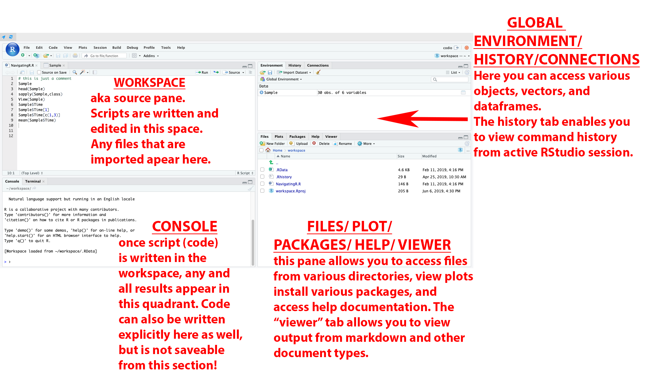
The following link shows what each quadrant in the RStudio IDE represents:
https://www.leonshpaner.com/teaching/post/rstudio/r_rstudio_installation/rstudio_workspace.png
Let’s talk about RStudio first, starting with the basics of R.
Table of Contents
- General (Console) Operations
- Determining and Setting The Current Working Directory
- Installing Packages
- Creating Objects
- Import Data From Flat CSV File
- Data Structures
- Sorting Data
- Handling #NA Values
- Inspecting #NA Values
- Basic Statistics
- Simulating a Normal Distribution
- Plots
- Basic Modeling
- Basic Modeling with Cross-Validation in R
General (Console) Operations
In R, we can simply type commands in the console window and hit “enter.” This is how they are executed. For example, R can be used as a calculator.
2 + 2## [1] 43 * 3## [1] 9sqrt(9)## [1] 3log10(100)## [1] 2What is a string?
A string is simply any open alpha/alphanumeric text characters surrounded by either single quotation marks or double quotation marks, with no preference assigned for either single or double quotation marks, with a print statement being called prior to the strings. For example,
print('This is a string.')## [1] "This is a string."print( "This is also a string123.")## [1] "This is also a string123."Determining and Setting The Current Working Directory
The importance of determining and setting the working directory cannot be stressed enough. Obtain the path to the working directory by running the getwd() function. Set the working directory by running the setwd("...") function, filling the parentheses inside with the correct path.
getwd()
setwd()
Installing Packages
To install a package or library, simply type in install.packages('package_name).
For the following exercises, let us ensure that we have installed the following packages:
# psychological library as extension for statistical tools install.packages(‘psych’)
# for reading rect. data (i.e., 'csv', 'tsv', and 'fwf') install.packages(“readr”)
# additional library for summarizing data install.packages(‘summarytools’)
# classification and regression training (modeling) install.packages(‘caret’)
# other miscellaneous function install.packages(‘e1071’)
# for classification and decision trees install.packages(‘rpart’)
# for plotting classification and decision trees install.packages(‘rpart.plot’)
# methods for cluster analysis install.packages(“cluster”)
# clustering algorithms & visualization install.packages(‘factoextra’)
To read the documentation for any given library, simply put a “?” before the library name and press “enter.” For example,
library(summarytools) # load the library first
# ?summarytools # then view the documentation
This will open the documentation in the ‘Files, Plots, Packages. Help, Viewer’ pane.
Creating Objects:
<- : assignment in R. Shortcut: "Alt + -" on Windows or "Option + -" on Mac.
var1 <- c(0, 1, 2, 3)Differences Between “=” and “<-”
Whereas "=" sign can also be used for assignment in R, it is best suited for specifying field equivalents (i.e., number of rows, columns, etc.). For example, let us take the following dataframe with 4 rows and 3 columns. Here, we specify A=4 and B=3 as follows:
dataframe_1 <- c(A = 4, B = 3)
dataframe_1
## A B
## 4 3If we specify A <- 4, and B <- 3 instead, A and B will effectively evaluate to those respective values as opposed to listing them in those respective columns. Let us take a look:
dataframe_2 <- c(A <- 4, B <- 3)
dataframe_2
## [1] 4 3Import Data From Flat CSV File
Assuming that your file is located in the same working directory that you have specified at the onset of this tutorial/workshop, make an assignment to a new variable (i.e., ex_csv) and call read.csv() in the following generalized format
For Windows users:
ex_csv_1 <- read.csv(choose.files(), header = T, quote = “’”)
# for macOS users
# example1.6 = read.csv(file.choose(), header = T, quote = "'")
The choose.files(), file.choose() function calls, respectively. allow the user to locate the file on their local drive, regardless of the working directory. That being said, there is more than one way to read in a .csv file. It does not have to exist on the local machine. If the file exists on the cloud, the path (link) can be parsed into the read.csv() function call as a string.
Now, let us print what is contained in var 1
print(var1)## [1] 0 1 2 3or we can simply call var1
var1## [1] 0 1 2 3Let us assign a variable to our earlier calculation and call the variable.
two <- 2+2
two
## [1] 4Any object (variable, vector, matrix, etc.) that is created is stored in the R workspace. From time to time, it is best practice to clear certain unused elements from the workspace so that it does not congest the memory.
rm(two)When we proceed to type in two, we will see that there is an error, confirming that the variable has been removed from the workspace.
There are 4 main data types in R: numeric, character, factor, and logical. There are data classes. Numeric variables includes integers and decimals.
num <- 12.6
num
## [1] 12.6Character (includes characters and strings):
char <- "Male"
char
## [1] "Male"Factor (ordinal/categorical data)”
gender <- as.factor(char)
gender
## [1] Male
## Levels: MaleLogical()
TRUE ## [1] TRUEFALSE## [1] FALSET # abbreviation also works for Boolean object## [1] TRUEF## [1] FALSETRUE * 7## [1] 7FALSE * 7## [1] 0Data Structures
What is a variable?
A variable is a container for storing a data value, exhibited as a reference to “to an object in memory which means that whenever a variable is assigned # to an instance, it gets mapped to that instance. A variable in R can store a vector, a group of vectors or a combination of many R objects” (GeeksforGeeks, 2020).
There are 3 most important data structures in R: vector, matrix, and dataframe.
Vector: the most basic type of data structure within R; contains a series of values of the same data class. It is a “sequence of data elements” (Thakur, 2018).
Matrix: a 2-dimensional version of a vector. Instead of only having a single row/list of data, we have rows and columns of data of the same data class.
Dataframe: the most important data structure for data science. Think of dataframe as loads of vectors pasted together as columns. Columns in a dataframe can be of different data class, but values within the same column must be the same data class.
The c() function is to R what concatenate() is to excel. For example,
vector_1 <- c(2,3,5)
vector_1
## [1] 2 3 5Similarly, a vector of logical values will contain the following.
vector_2 <- c(TRUE, FALSE, TRUE, FALSE, FALSE)
vector_2
## [1] TRUE FALSE TRUE FALSE FALSETo determine the number of members inside any given vector, we apply the length() function call on the vector as follows:
length(c(TRUE, FALSE, TRUE, FALSE, FALSE))## [1] 5or, since we already assigned this to a data frame named vector_2, we can simply call length of vector_2 as follows:
length(vector_2)## [1] 5Let’s say for example, that we want to access the third element of vector_1. We can do so as follows:
vector_1[3]## [1] 5What if we want to access all elements within the dataframe except for the first one? To this end, we use the "-" symbol as follows:
vector_1[-1]## [1] 3 5Let us create a longer arbitrary vector so we can illustrate some further examples.
vector_3 <- c(1,3,5,7,9,20,2,8,10,35,76,89,207)To access the first, fifth, and ninth elements of this dataframe. To this end, we can do the following:
vector_3[c(1,5,9)]## [1] 1 9 10To access all elements within a specified range, specify the exact range using the ":" separator as follows:
vector_3[3:11]## [1] 5 7 9 20 2 8 10 35 76Let us create a mock dataframe for five fictitious individuals representing different ages, and departments at a research facility.
Name <- c('Jack', 'Kathy', 'Latesha', 'Brandon', 'Alexa', 'Jonathan', 'Joshua',
          'Emily', 'Matthew', 'Anthony', 'Margaret', 'Natalie')

Age <- c(47, 41, 23, 55, 36, 54, 48, 23, 22, 27, 37, 43)
Experience <- c(7,5,9,3,11,6,8,9,5,2,1,4)

Position <- c('Economist', 'Director of Operations', 'Human Resources',
              'Admin. Assistant', 'Data Scientist', 'Admin. Assistant',
              'Account Manager', 'Account Manager', 'Attorney', 'Paralegal',
              'Data Analyst', 'Research Assistant')

df <- data.frame(Name, Age, Experience, Position)
df
## Name Age Experience Position
## 1 Jack 47 7 Economist
## 2 Kathy 41 5 Director of Operations
## 3 Latesha 23 9 Human Resources
## 4 Brandon 55 3 Admin. Assistant
## 5 Alexa 36 11 Data Scientist
## 6 Jonathan 54 6 Admin. Assistant
## 7 Joshua 48 8 Account Manager
## 8 Emily 23 9 Account Manager
## 9 Matthew 22 5 Attorney
## 10 Anthony 27 2 Paralegal
## 11 Margaret 37 1 Data Analyst
## 12 Natalie 43 4 Research AssistantLet us examine the structure of the dataframe.
str(df)## 'data.frame': 12 obs. of 4 variables:
## $ Name : chr "Jack" "Kathy" "Latesha" "Brandon" ...
## $ Age : num 47 41 23 55 36 54 48 23 22 27 ...
## $ Experience: num 7 5 9 3 11 6 8 9 5 2 ...
## $ Position : chr "Economist" "Director of Operations" "Human Resources" "Admin. Assistant" ...Let us examine the dimensions of the dataframe (number of rows and columns, respectively).
dim(df)## [1] 12 4Sorting Data
Let us say that now we want to sort this dataframe in order of age (youngest to oldest).
df_age <- df[order(Age),]
df_age
## Name Age Experience Position
## 9 Matthew 22 5 Attorney
## 3 Latesha 23 9 Human Resources
## 8 Emily 23 9 Account Manager
## 10 Anthony 27 2 Paralegal
## 5 Alexa 36 11 Data Scientist
## 11 Margaret 37 1 Data Analyst
## 2 Kathy 41 5 Director of Operations
## 12 Natalie 43 4 Research Assistant
## 1 Jack 47 7 Economist
## 7 Joshua 48 8 Account Manager
## 6 Jonathan 54 6 Admin. Assistant
## 4 Brandon 55 3 Admin. AssistantNow, if we want to sort experience by descending order while keeping age sorted according to previous specifications, we can do the following:
df_age_exp <- df[order(Age, Experience),]
df_age_exp
## Name Age Experience Position
## 9 Matthew 22 5 Attorney
## 3 Latesha 23 9 Human Resources
## 8 Emily 23 9 Account Manager
## 10 Anthony 27 2 Paralegal
## 5 Alexa 36 11 Data Scientist
## 11 Margaret 37 1 Data Analyst
## 2 Kathy 41 5 Director of Operations
## 12 Natalie 43 4 Research Assistant
## 1 Jack 47 7 Economist
## 7 Joshua 48 8 Account Manager
## 6 Jonathan 54 6 Admin. Assistant
## 4 Brandon 55 3 Admin. AssistantHandling #NA Values
NA (not available) refers to missing values. What if our dataset has missing values? How should we handle this scenario? For example, age has some missing values.
Name_2 <- c('Jack', 'Kathy', 'Latesha', 'Brandon', 'Alexa', 'Jonathan', 'Joshua',
            'Emily', 'Matthew', 'Anthony', 'Margaret', 'Natalie')

Age_2 <- c(47, NA, 23, 55, 36, 54, 48, NA, 22, 27, 37, 43)
Experience_2 <- c(7,5,9,3,11,6,8,9,5,2,1,4)

Position_2 <- c('Economist', 'Director of Operations', 'Human Resources',
                'Admin. Assistant', 'Data Scientist', 'Admin. Assistant',
                'Account Manager', 'Account Manager', 'Attorney', 'Paralegal',
                'Data Analyst', 'Research Assistant')

df_2 <- data.frame(Name_2, Age_2, Experience_2, Position_2)
df_2
## Name_2 Age_2 Experience_2 Position_2
## 1 Jack 47 7 Economist
## 2 Kathy NA 5 Director of Operations
## 3 Latesha 23 9 Human Resources
## 4 Brandon 55 3 Admin. Assistant
## 5 Alexa 36 11 Data Scientist
## 6 Jonathan 54 6 Admin. Assistant
## 7 Joshua 48 8 Account Manager
## 8 Emily NA 9 Account Manager
## 9 Matthew 22 5 Attorney
## 10 Anthony 27 2 Paralegal
## 11 Margaret 37 1 Data Analyst
## 12 Natalie 43 4 Research AssistantInspecting #NA Values
is.na(df_2) # returns a Boolean matrix (True or False)## Name_2 Age_2 Experience_2 Position_2
## [1,] FALSE FALSE FALSE FALSE
## [2,] FALSE TRUE FALSE FALSE
## [3,] FALSE FALSE FALSE FALSE
## [4,] FALSE FALSE FALSE FALSE
## [5,] FALSE FALSE FALSE FALSE
## [6,] FALSE FALSE FALSE FALSE
## [7,] FALSE FALSE FALSE FALSE
## [8,] FALSE TRUE FALSE FALSE
## [9,] FALSE FALSE FALSE FALSE
## [10,] FALSE FALSE FALSE FALSE
## [11,] FALSE FALSE FALSE FALSE
## [12,] FALSE FALSE FALSE FALSEsum(is.na(df_2)) # sums up all of the NA values in the dataframe ## [1] 2df_2[!complete.cases(df_2),] # we can provide a list of rows with missing data## Name_2 Age_2 Experience_2 Position_2
## 2 Kathy NA 5 Director of Operations
## 8 Emily NA 9 Account ManagerWe can delete the rows with missing values by making an na.omit() function call in the following manner:
df_2_na_omit <- na.omit(df_2)
df_2_na_omit
## Name_2 Age_2 Experience_2 Position_2
## 1 Jack 47 7 Economist
## 3 Latesha 23 9 Human Resources
## 4 Brandon 55 3 Admin. Assistant
## 5 Alexa 36 11 Data Scientist
## 6 Jonathan 54 6 Admin. Assistant
## 7 Joshua 48 8 Account Manager
## 9 Matthew 22 5 Attorney
## 10 Anthony 27 2 Paralegal
## 11 Margaret 37 1 Data Analyst
## 12 Natalie 43 4 Research AssistantOr we can use complete.cases() to subset only those rows that do not have missing values:
df_2[complete.cases(df_2), ]## Name_2 Age_2 Experience_2 Position_2
## 1 Jack 47 7 Economist
## 3 Latesha 23 9 Human Resources
## 4 Brandon 55 3 Admin. Assistant
## 5 Alexa 36 11 Data Scientist
## 6 Jonathan 54 6 Admin. Assistant
## 7 Joshua 48 8 Account Manager
## 9 Matthew 22 5 Attorney
## 10 Anthony 27 2 Paralegal
## 11 Margaret 37 1 Data Analyst
## 12 Natalie 43 4 Research AssistantWhat if we receive a dataframe that, at a cursory glance, warehouses numerical values where we see numbers, but when running additional operations on the dataframe, we discover that we cannot conduct numerical exercises with columns that appear to have numbers. This is exactly why it is of utmost importance for us to always inspect the structure of the dataframe using the str() function call. Here is an example of the same dataframe with altered data types.
Name_3 <- c('Jack', 'Kathy', 'Latesha', 'Brandon', 'Alexa', 'Jonathan', 'Joshua',
            'Emily', 'Matthew', 'Anthony', 'Margaret', 'Natalie')

Age_3 <- c('47', '41', '23', '55', '36', '54', '48', '23', '22', '27', '37', '43')

Experience_3 <- c(7,5,9,3,11,6,8,9,5,2,1,4)

Position_3 <- c('Economist', 'Director of Operations', 'Human Resources',
                'Admin. Assistant', 'Data Scientist', 'Admin. Assistant',
                'Account Manager', 'Account Manager', 'Attorney', 'Paralegal',
                'Data Analyst', 'Research Assistant')

df_3 <- data.frame(Name_3, Age_3, Experience_3, Position_3)
Notice how Age is now expressed as a character data type, whereas Experience still shows as a numeric datatype.
str(df_3,
    strict.width = 'wrap')
## 'data.frame': 12 obs. of 4 variables:
## $ Name_3 : chr "Jack" "Kathy" "Latesha" "Brandon" ...
## $ Age_3 : chr "47" "41" "23" "55" ...
## $ Experience_3: num 7 5 9 3 11 6 8 9 5 2 ...
## $ Position_3 : chr "Economist" "Director of Operations" "Human Resources"
## "Admin. Assistant" ...Let us convert Age back to numeric using the as.numeric() function, and re-examine the dataframe.
df_3$Age_3 <- as.numeric(df_3$Age_3)
str(df_3, strict.width = 'wrap')
## 'data.frame': 12 obs. of 4 variables:
## $ Name_3 : chr "Jack" "Kathy" "Latesha" "Brandon" ...
## $ Age_3 : num 47 41 23 55 36 54 48 23 22 27 ...
## $ Experience_3: num 7 5 9 3 11 6 8 9 5 2 ...
## $ Position_3 : chr "Economist" "Director of Operations" "Human Resources"
## "Admin. Assistant" ...We can also convert experience from numeric to character/categorical data as follows:
options(width = 60)
df_3$Experience_3 <- as.character(df_3$Experience_3)
str(df_3, width = 60, strict.width = 'wrap')
## 'data.frame': 12 obs. of 4 variables:
## $ Name_3 : chr "Jack" "Kathy" "Latesha" "Brandon" ...
## $ Age_3 : num 47 41 23 55 36 54 48 23 22 27 ...
## $ Experience_3: chr "7" "5" "9" "3" ...
## $ Position_3 : chr "Economist" "Director of Operations"
## "Human Resources" "Admin. Assistant" ...Basic Statistics
Setting the seed
First, let us discuss the importance of setting a seed. Setting a seed to a specific yet arbitrary value in R ensures the reproducibility of results. It is always best practice to use the same assigned seed throughout the entire experiment. Setting the seed to this arbitrary number (of any length) will guarantee exactly the same output across all R sessions and users, respectively.
Let us create a new data frame of numbers 1 - 100.
mystats <- c(1:100)and go over the basic statistical functions
mean(mystats) # mean of the vector## [1] 50.5median(mystats) # median of the vector## [1] 50.5min(mystats) # minimum of the vector## [1] 1max(mystats) # maximum of the vector## [1] 100range(mystats) # range of the vector## [1] 1 100sum(mystats) # sum of the vector## [1] 5050sd(mystats) # standard deviation of the vector## [1] 29.01149class(mystats) # return data class of the vector## [1] "integer"length(mystats) # the length of the vector## [1] 100# summary of the dataset
summary(mystats) ## Min. 1st Qu. Median Mean 3rd Qu. Max.
## 1.00 25.75 50.50 50.50 75.25 100.00To use an installed library, we must open that library with the following library() function call
library(psych)For example, the psych library uses the describe() function call to give us an alternate perspective int the summary statistics of the data.
describe(mystats)## vars n mean sd median trimmed mad min max range
## X1 1 100 50.5 29.01 50.5 50.5 37.06 1 100 99
## skew kurtosis se
## X1 0 -1.24 2.9library(summarytools)
dfSummary(mystats, plain.ascii = FALSE,
style = 'grid',
graph.magnif = 0.85,
varnumbers = FALSE,
valid.col = FALSE,
tmp.img.dir = "/tmp",
method='pandoc')## mystats was converted to a data frame## temporary images written to 'C:\tmp'## ### Data Frame Summary
## #### mystats
## **Dimensions:** 100 x 1
## **Duplicates:** 0
##
## +-----------+------------------------+----------------------+----------------------+---------+
## | Variable | Stats / Values | Freqs (% of Valid) | Graph | Missing |
## +===========+========================+======================+======================+=========+
## | mystats\ | Mean (sd) : 50.5 (29)\ | 100 distinct values\ |  | 0\ |
## | [integer] | min < med < max:\ | (Integer sequence) | | (0.0%) |
## | | 1 < 50.5 < 100\ | | | |
## | | IQR (CV) : 49.5 (0.6) | | | |
## +-----------+------------------------+----------------------+----------------------+---------+Simulating a Normal Distribution
Now, We will use the rnorm() function to simulate a vector of 100 random normally distributed data with a mean of 50, and a standard deviation of 10.
set.seed(222) # set.seed() for reproducibility
norm_vals <- rnorm(n = 100, mean = 50, sd = 10)
norm_vals
## [1] 64.87757 49.98108 63.81021 46.19786 51.84136 47.53104
## [7] 37.84439 65.61405 54.27310 37.98976 60.52458 36.94936
## [13] 43.07392 56.02649 48.02247 38.14125 29.94487 50.07510
## [19] 55.19490 42.53705 57.26455 57.13657 43.49937 64.98696
## [25] 35.64172 28.38682 53.95220 46.05166 46.90242 63.30827
## [31] 41.82571 56.75893 47.84519 48.85350 47.97735 54.06493
## [37] 56.56772 51.06191 48.15603 59.46034 52.02387 54.95101
## [43] 44.30645 61.19294 72.09078 53.17183 40.64703 58.13662
## [49] 46.24635 53.33100 55.94415 55.20868 40.47956 37.72315
## [55] 47.97593 60.59120 53.81779 62.39694 53.16777 39.56622
## [61] 38.51764 62.31145 57.89215 57.48845 50.57476 58.42951
## [67] 51.99859 64.51171 45.39840 22.25533 50.56489 49.38629
## [73] 38.18032 24.70833 58.13577 52.62389 49.37494 56.71735
## [79] 50.27176 55.35603 56.89548 38.00871 37.60845 52.13186
## [85] 35.42848 48.74239 55.44208 57.20830 34.28810 60.97272
## [91] 46.67537 56.16393 55.08799 66.86555 53.79547 52.35471
## [97] 54.24988 38.15064 43.56390 50.52614Plots
Stem-and-leaf
Let’s make a Simple stem-and-leaf plot. Here, we call the stem() function as follows:
stem(norm_vals)##
## The decimal point is 1 digit(s) to the right of the |
##
## 2 | 2
## 2 | 58
## 3 | 04
## 3 | 567888888889
## 4 | 001233344
## 4 | 5666778888889999
## 5 | 0001111222223333444444
## 5 | 5555556667777777788889
## 6 | 11112234
## 6 | 55567
## 7 | 2We can plot a histogram of these norm_vals in order to inspect their distribution from a purely graphical standpoint. R uses the built-in hist() function to accomplish this task. Let us now plot the histogram.
Histograms
hist(norm_vals)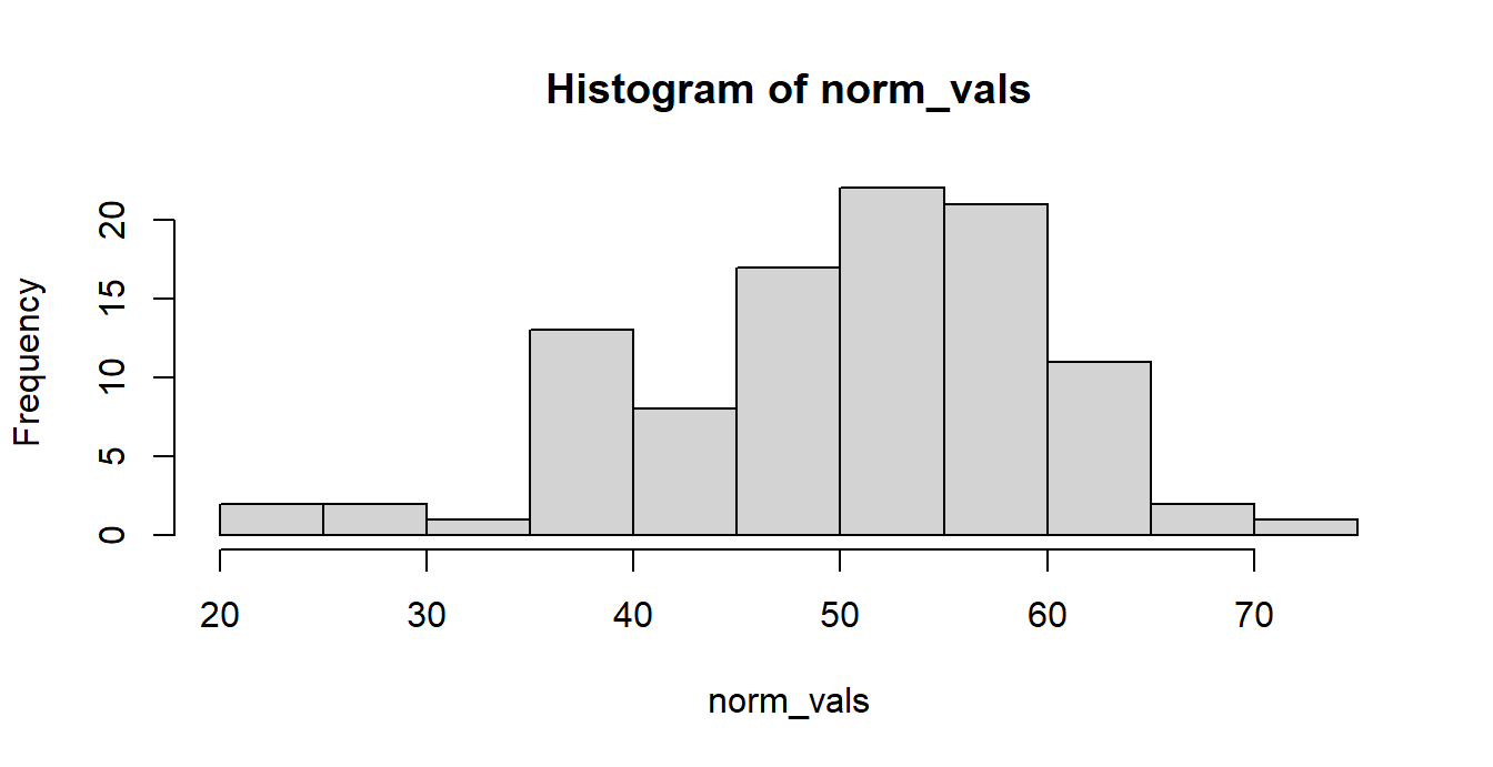
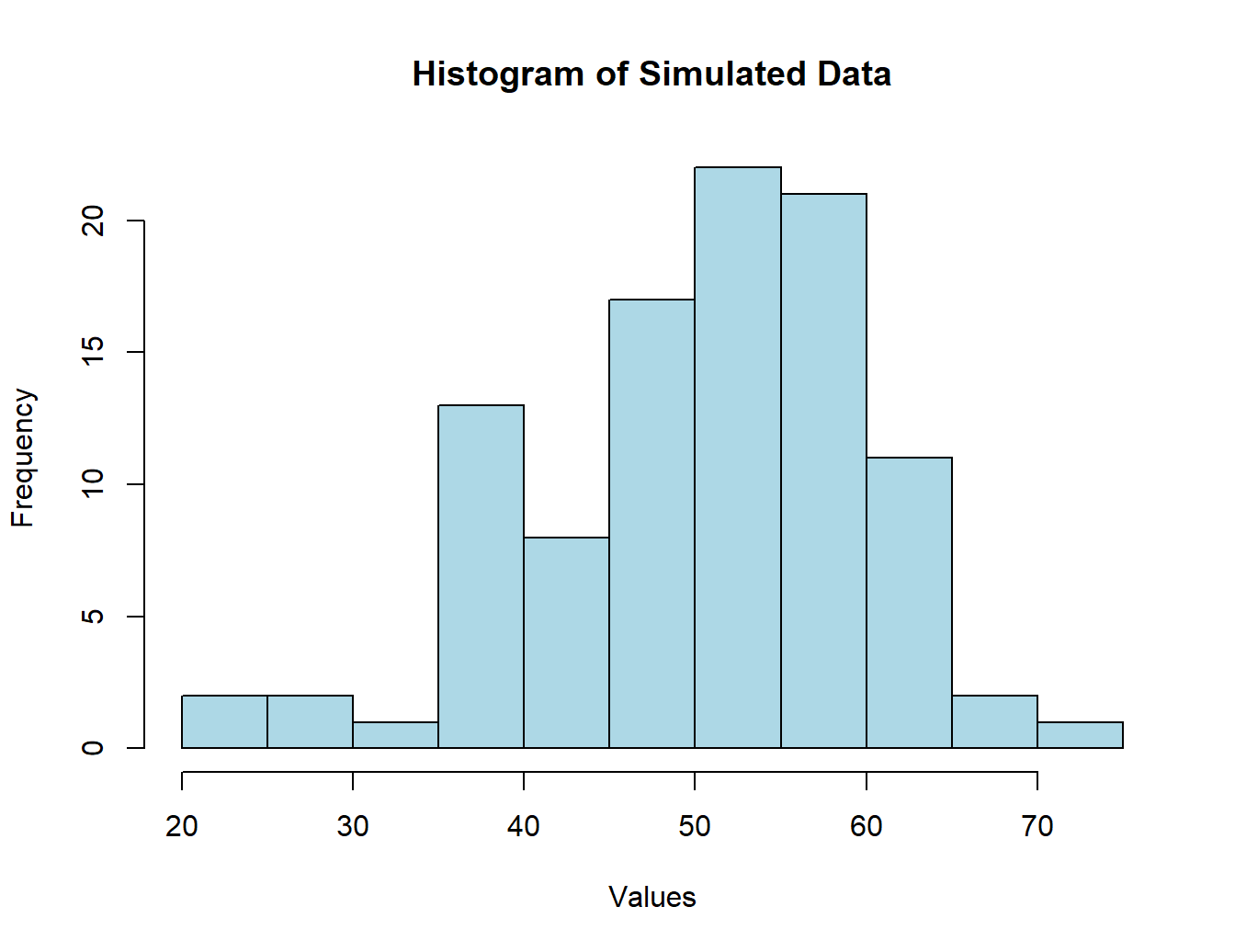
Our title, x-axis, and y-axis labels are given to us by default. However, let us say that we want to change all of them to our desired specifications. To this end, we can parse in and control the following parameters:
hist(norm_vals,
     col = 'lightblue', # specify the color
     xlab = 'Values', # specify the x-axis label
     ylab = 'Frequency', # specify the y-axis label
     main = 'Histogram of Simulated Data', # specify the new title
     )
Boxplots
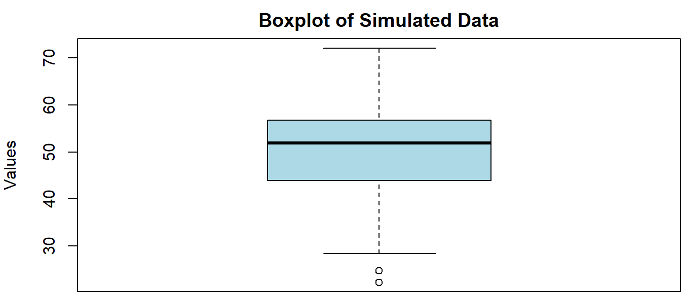
Similarly, we can make a boxplot in base R using the boxplot() function call as follows:
par(mar = c(0,4,2,0))
boxplot(norm_vals,
        col = 'lightblue', # specify the color
        ylab = 'Values', # specify the y-axis label
        main = 'Boxplot of Simulated Data' # specify the new title
        )
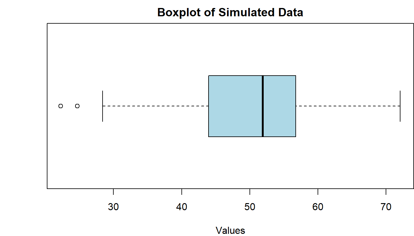
Now, let us pivot the boxplot by parsing in the horizontal = TRUE parameter:
par(mar = c(4,4,2,0))
boxplot(norm_vals, horizontal = TRUE,
        col = 'lightblue', # specify the color
        xlab = 'Values', # specify the x-axis label
        main = 'Boxplot of Simulated Data' # specify the new title
        )
Scatter Plots
To make a simple scatter plot, we will simply call the plot() function on the same dataframe as follows:
plot(norm_vals,
     main = 'Scatter Plot of Simulated Data',
     pch = 20, # plot character - in this case default (circle)
     xlab = 'Index',
     ylab = 'Value')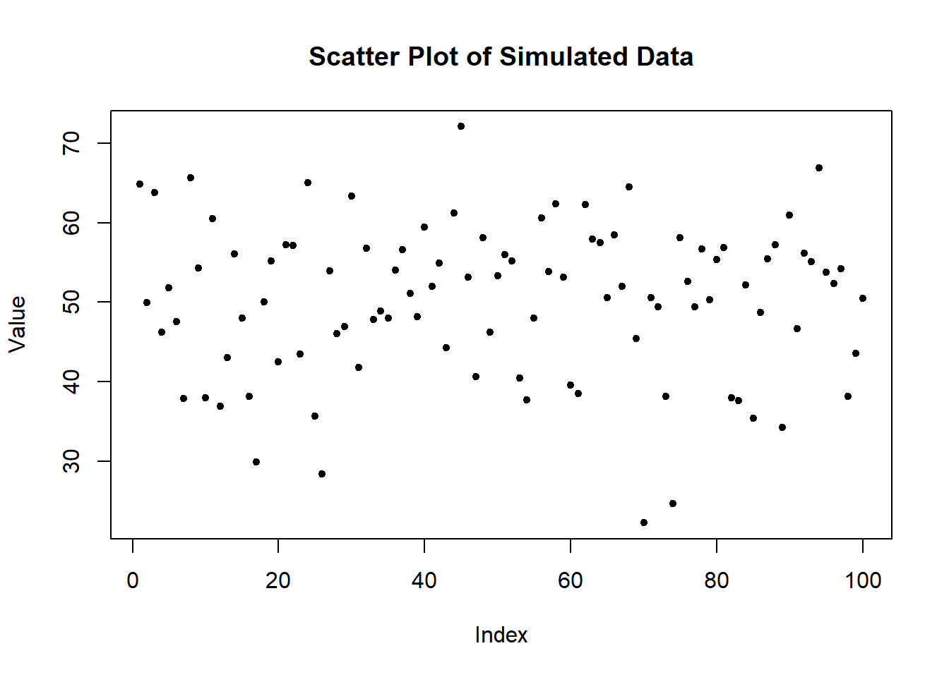
Quantile-Quantile Plot
Let us create a vector for the next example data and generate a normal quantile plot.
quant_ex <- c(48.30, 49.03, 50.24, 51.39, 48.74, 51.55, 51.17, 49.87, 50.16,
              49.80, 46.83, 48.48, 52.24, 50.01, 49.50, 49.97, 48.56, 50.87)

qqnorm(quant_ex)

qqline(quant_ex) # adding a theoretical Q-Q line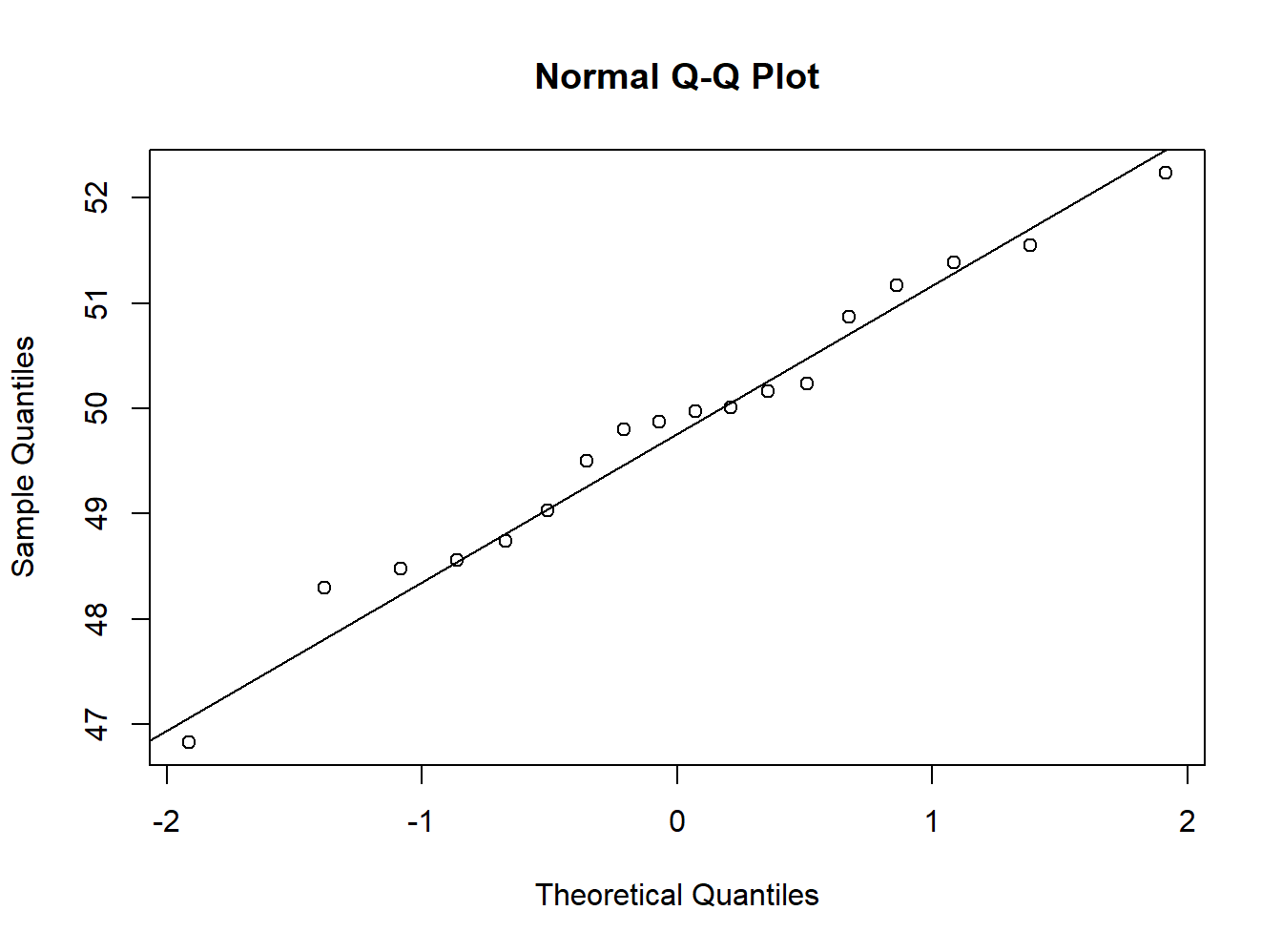
Skewness and Box-Cox Transformation
From statistics, let us recall that if the mean is greater than the median, the distribution will be positively skewed. Conversely, if the median is greater than the mean, or the mean is less than the median, the distribution will be negatively skewed. Let us examine the exact skewness of our distribution.
# Test skewness by looking at mean and median relationship
mean_norm_vals <- round(mean(norm_vals),0)
median_norm_vals <- round(median(norm_vals),0)
distribution <- data.frame(mean_norm_vals,
                           median_norm_vals)
distribution
## mean_norm_vals median_norm_vals
## 1 50 52library(e1071)
skewness(norm_vals) # apply `skewness()` function from the e1071 library## [1] -0.497993# Applying Box-Cox Transformation on skewed variable
library(caret)## Loading required package: ggplot2##
## Attaching package: 'ggplot2'## The following object is masked _by_ '.GlobalEnv':
##
## Position## The following objects are masked from 'package:psych':
##
## %+%, alpha## Loading required package: latticetrans <- preProcess(data.frame(norm_vals), method=c("BoxCox"))
trans## Created from 100 samples and 1 variables
##
## Pre-processing:
## - Box-Cox transformation (1)
## - ignored (0)
##
## Lambda estimates for Box-Cox transformation:
## 1.8Basic Modeling
Linear Regression
Let us set up an example dataset for the following modeling endeavors.
# independent variables (x's):

# X1
Hydrogen <- c(.18,.20,.21,.21,.21,.22,.23,.23,.24,.24,.25,.28,.30,.37,.31,.90,
              .81,.41,.74,.42,.37,.49,.07,.94,.47,.35,.83,.61,.30,.61,.54)

# X2
Oxygen <- c(.55,.77,.40,.45,.62,.78,.24,.47,.15,.70,.99,.62,.55,.88,.49,.36,.55,
            .42,.39,.74,.50,.17,.18,.94,.97,.29,.85,.17,.33,.29,.85)

# X3
Nitrogen <- c(.35,.48,.31,.75,.32,.56,.06,.46,.79,.88,.66,.04,.44,.61,.15,.48,
              .23,.90,.26,.41,.76,.30,.56,.73,.10,.01,.05,.34,.27,.42,.83)

# there is always one dependent variable (target, response, y)
Gas_Porosity <- c(.46,.70,.41,.45,.55,.44,.24,.47,.22,.80,.88,.70,.72,.75,.16,
                  .15,.08,.47,.59,.21,.37,.96,.06,.17,.10,.92,.80,.06,.52,.01,.3)
Simple Linear Regression
Prior to partaking in linear regression, it is best practice to examine correlation from a strictly visual perspective visa vie scatterplot as follows:
plot(Hydrogen,
     Gas_Porosity,
     main = "Scatter Plot - Gas Porosity vs. Hydrogen Content",
     xlab = "Hydrogen Content",
     ylab = "Gas Porosity",
     pch=16,
     col="blue")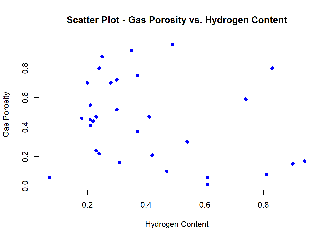
Now, let’s find the correlation coefficient, r.
r1 <- cor(Hydrogen, Gas_Porosity)
r1
## [1] -0.2424314Now we can set-up the linear model between one independent variable and one dependent variable.
simple_linear_mod <- data.frame(Hydrogen, Gas_Porosity)By the correlation coefficient r you will see that there exists a relatively moderate (positive) relationship. Let us now build a simple linear model from this dataframe.
lm_model1 <- lm(Gas_Porosity ~ Hydrogen, data = simple_linear_mod)
summary(lm_model1)
##
## Call:
## lm(formula = Gas_Porosity ~ Hydrogen, data = simple_linear_mod)
##
## Residuals:
## Min 1Q Median 3Q Max
## -0.48103 -0.23564 -0.04983 0.23346 0.54258
##
## Coefficients:
## Estimate Std. Error t value Pr(>|t|)
## (Intercept) 0.5616 0.1018 5.516 6.06e-06 ***
## Hydrogen -0.2943 0.2187 -1.346 0.189
## ---
## Signif. codes:
## 0 '***' 0.001 '**' 0.01 '*' 0.05 '.' 0.1 ' ' 1
##
## Residual standard error: 0.2807 on 29 degrees of freedom
## Multiple R-squared: 0.05877, Adjusted R-squared: 0.02632
## F-statistic: 1.811 on 1 and 29 DF, p-value: 0.1888Notice how the p-value for hydrogen content is 0.189, which lacks statistical significance when compared to the alpha value of 0.05 (at the 95% confidence level). Moreover, the R-Squared value of .05877 suggests that roughly 6% of the variance for gas propensity is explained by hydrogen content.
# we can make the same scatter plot, but this time with a best fit line
plot(Hydrogen,
     Gas_Porosity,
     main = "Scatter Plot - Gas Porosity vs. Hydrogen Content",
     xlab = "Hydrogen Content",
     ylab = "Gas Porosity",
     pch=16,
     col="blue",
abline(lm_model1, col="red")) 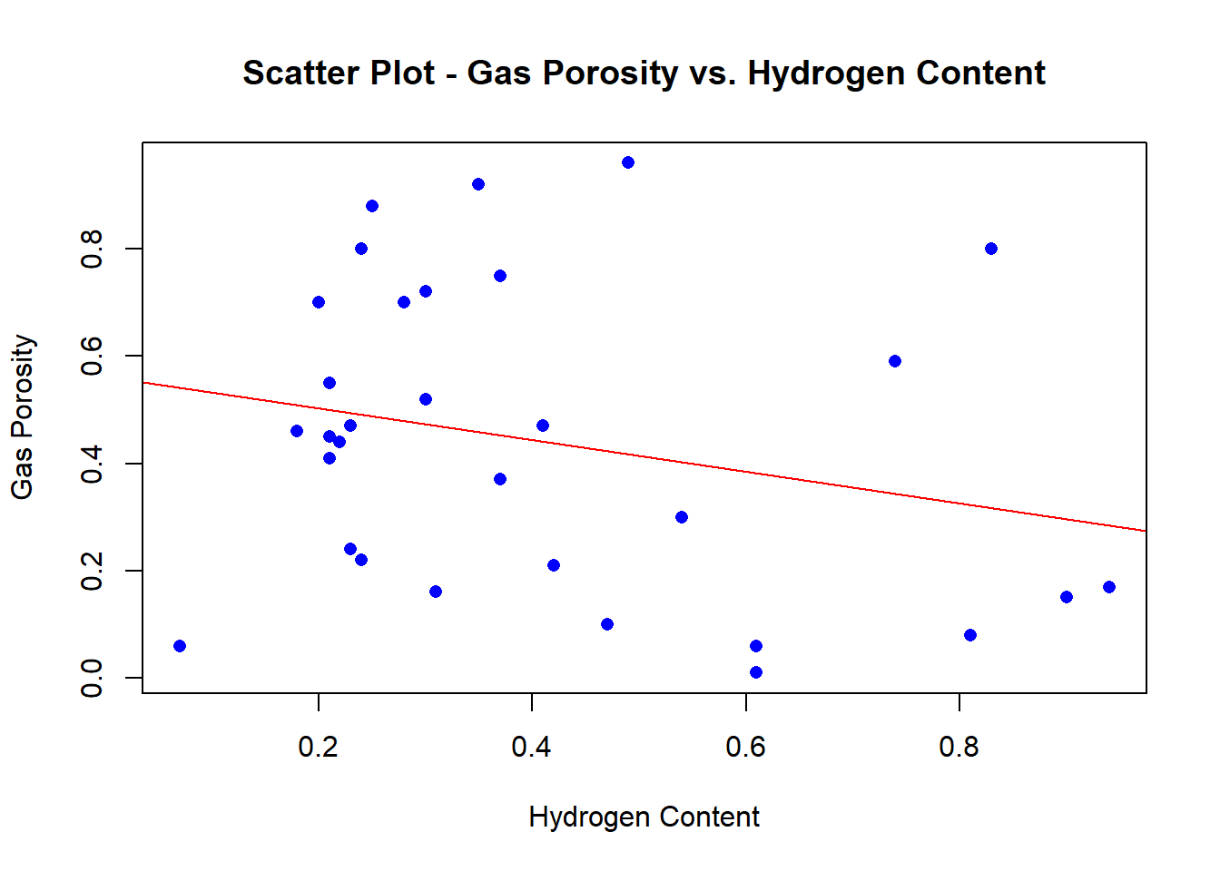
Multiple Linear Regression
To account for all independent (x) variables in the model, let us set up the model in a dataframe:
multiple_linear_mod <- data.frame(Hydrogen, Oxygen, Nitrogen, Gas_Porosity)We can make additional scatter plots:
# gas porosity vs. oxygen
plot(Oxygen,
     Gas_Porosity,
     main = "Scatter Plot - Gas Porosity vs. Oxygen Content",
     xlab = "Oxygen Content",
     ylab = "Gas Porosity",
     pch=16,
     col="blue")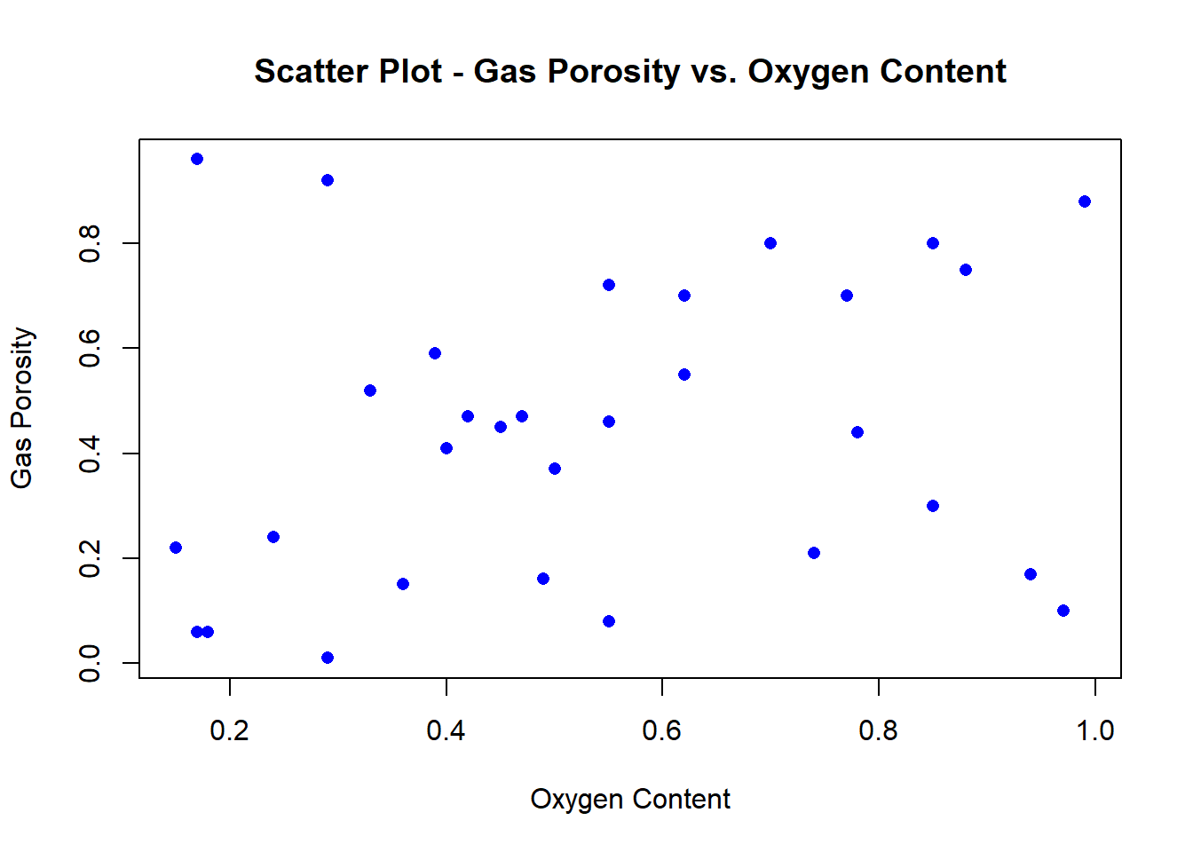
# gas porosity vs. nitrogen content
plot(Nitrogen,
     Gas_Porosity,
     main = "Scatter Plot - Gas Porosity vs. Oxygen Content",
     xlab = "Oxygen Content",
     ylab = "Gas Porosity",
     pch=16,
     col="blue")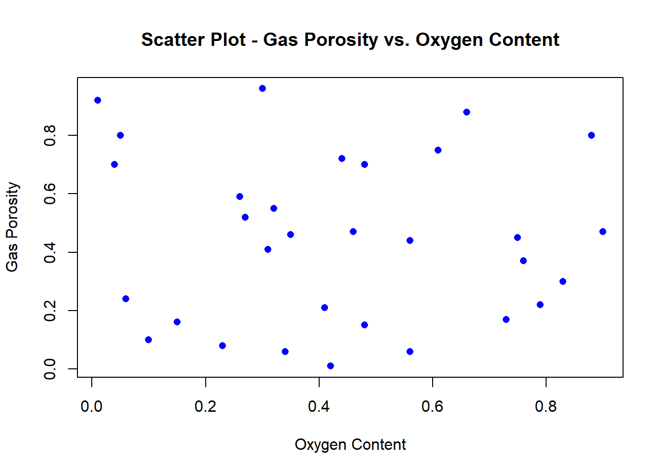
and lastly, we can build a multiple linear model from these 3 independent variables:
lm_model2 <- lm(Gas_Porosity ~ Hydrogen + Oxygen + Nitrogen,
                data = multiple_linear_mod)
summary(lm_model2)
##
## Call:
## lm(formula = Gas_Porosity ~ Hydrogen + Oxygen + Nitrogen, data = multiple_linear_mod)
##
## Residuals:
## Min 1Q Median 3Q Max
## -0.49593 -0.18800 -0.02835 0.17512 0.63885
##
## Coefficients:
## Estimate Std. Error t value Pr(>|t|)
## (Intercept) 0.4853 0.1605 3.024 0.00542 **
## Hydrogen -0.3536 0.2210 -1.600 0.12122
## Oxygen 0.2998 0.2036 1.473 0.15241
## Nitrogen -0.1395 0.1970 -0.708 0.48496
## ---
## Signif. codes:
## 0 '***' 0.001 '**' 0.01 '*' 0.05 '.' 0.1 ' ' 1
##
## Residual standard error: 0.2788 on 27 degrees of freedom
## Multiple R-squared: 0.1352, Adjusted R-squared: 0.03906
## F-statistic: 1.407 on 3 and 27 DF, p-value: 0.2624Logistic Regression
Whereas in linear regression, it is necessary to have a quantitative and continuous target variable, logistic regression is part of the generalized linear model series that has a categorical (often binary) target (outcome) variable. For example, let us say we want to predict grades for mathematics courses taught at a university.
So, we have the following example dataset:
# grades for calculus 1
calculus1 <- c(56,80,10,8,20,90,38,42,57,58,90,2,34,84,19,74,13,67,84,31,82,67,
               99,76,96,59,37,24,3,57,62)

# grades for calculus 2
calculus2 <- c(83,98,50,16,70,31,90,48,67,78,55,75,20,80,74,86,12,100,63,36,91,
               19,69,58,85,77,5,31,57,72,89)

# grades for linear algebra
linear_alg <- c(87,90,85,57,30,78,75,69,83,85,90,85,99,97, 38,95,10,99,62,47,17,
                31,77,92,13,44,3,83,21,38,70)

# students passing/fail
pass_fail <- c('P','F','P','F','P','P','P','P','F','P','P','P','P','P','P','F',
               'P','P','P','F','F','F','P','P','P','P','P','P','P','P','P')
At this juncture, we cannot build a model with categorical values until and unless they are binarized using the ifelse() function call as follows. A passing score will be designated by a 1, and failing score with a respectively.
math_outcome <- ifelse(pass_fail=='P', 1, 0)
math_outcome
## [1] 1 0 1 0 1 1 1 1 0 1 1 1 1 1 1 0 1 1 1 0 0 0 1 1 1 1 1 1
## [29] 1 1 1logistic_model <- data.frame(calculus1,
calculus2,
linear_alg,
pass_fail,
math_outcome)
# examine data structures of the model
str(logistic_model) ## 'data.frame': 31 obs. of 5 variables:
## $ calculus1 : num 56 80 10 8 20 90 38 42 57 58 ...
## $ calculus2 : num 83 98 50 16 70 31 90 48 67 78 ...
## $ linear_alg : num 87 90 85 57 30 78 75 69 83 85 ...
## $ pass_fail : chr "P" "F" "P" "F" ...
## $ math_outcome: num 1 0 1 0 1 1 1 1 0 1 ...We can also specify glm instead of just lm as in linear regression example:
lm_model3 <- glm(math_outcome ~ calculus1 +
                                calculus2 +
                                linear_alg,
                 family = binomial(),
                 data = logistic_model)

summary(lm_model3)
##
## Call:
## glm(formula = math_outcome ~ calculus1 + calculus2 + linear_alg,
## family = binomial(), data = logistic_model)
##
## Coefficients:
## Estimate Std. Error z value Pr(>|z|)
## (Intercept) 1.132509 1.278396 0.886 0.376
## calculus1 -0.010621 0.016416 -0.647 0.518
## calculus2 0.006131 0.017653 0.347 0.728
## linear_alg 0.004902 0.014960 0.328 0.743
##
## (Dispersion parameter for binomial family taken to be 1)
##
## Null deviance: 33.118 on 30 degrees of freedom
## Residual deviance: 32.589 on 27 degrees of freedom
## AIC: 40.589
##
## Number of Fisher Scoring iterations: 4Decision Trees
Decision trees are valuable supplementary methods for tracing consequential outcomes diagrammatically.
We can plot the trajectory of the outcome using the rpart() function of the library(rpart) and library(rpart.plot), respectively.
library(rpart)
library(rpart.plot)
In favor of a larger dataset to illustrate the structure, function, and overall efficacy of decision trees in R, we will rely on the built-in mtcars dataset.
str(mtcars)## 'data.frame': 32 obs. of 11 variables:
## $ mpg : num 21 21 22.8 21.4 18.7 18.1 14.3 24.4 22.8 19.2 ...
## $ cyl : num 6 6 4 6 8 6 8 4 4 6 ...
## $ disp: num 160 160 108 258 360 ...
## $ hp : num 110 110 93 110 175 105 245 62 95 123 ...
## $ drat: num 3.9 3.9 3.85 3.08 3.15 2.76 3.21 3.69 3.92 3.92 ...
## $ wt : num 2.62 2.88 2.32 3.21 3.44 ...
## $ qsec: num 16.5 17 18.6 19.4 17 ...
## $ vs : num 0 0 1 1 0 1 0 1 1 1 ...
## $ am : num 1 1 1 0 0 0 0 0 0 0 ...
## $ gear: num 4 4 4 3 3 3 3 4 4 4 ...
## $ carb: num 4 4 1 1 2 1 4 2 2 4 ...mtcars## mpg cyl disp hp drat wt qsec vs
## Mazda RX4 21.0 6 160.0 110 3.90 2.620 16.46 0
## Mazda RX4 Wag 21.0 6 160.0 110 3.90 2.875 17.02 0
## Datsun 710 22.8 4 108.0 93 3.85 2.320 18.61 1
## Hornet 4 Drive 21.4 6 258.0 110 3.08 3.215 19.44 1
## Hornet Sportabout 18.7 8 360.0 175 3.15 3.440 17.02 0
## Valiant 18.1 6 225.0 105 2.76 3.460 20.22 1
## Duster 360 14.3 8 360.0 245 3.21 3.570 15.84 0
## Merc 240D 24.4 4 146.7 62 3.69 3.190 20.00 1
## Merc 230 22.8 4 140.8 95 3.92 3.150 22.90 1
## Merc 280 19.2 6 167.6 123 3.92 3.440 18.30 1
## Merc 280C 17.8 6 167.6 123 3.92 3.440 18.90 1
## Merc 450SE 16.4 8 275.8 180 3.07 4.070 17.40 0
## Merc 450SL 17.3 8 275.8 180 3.07 3.730 17.60 0
## Merc 450SLC 15.2 8 275.8 180 3.07 3.780 18.00 0
## Cadillac Fleetwood 10.4 8 472.0 205 2.93 5.250 17.98 0
## Lincoln Continental 10.4 8 460.0 215 3.00 5.424 17.82 0
## Chrysler Imperial 14.7 8 440.0 230 3.23 5.345 17.42 0
## Fiat 128 32.4 4 78.7 66 4.08 2.200 19.47 1
## Honda Civic 30.4 4 75.7 52 4.93 1.615 18.52 1
## Toyota Corolla 33.9 4 71.1 65 4.22 1.835 19.90 1
## Toyota Corona 21.5 4 120.1 97 3.70 2.465 20.01 1
## Dodge Challenger 15.5 8 318.0 150 2.76 3.520 16.87 0
## AMC Javelin 15.2 8 304.0 150 3.15 3.435 17.30 0
## Camaro Z28 13.3 8 350.0 245 3.73 3.840 15.41 0
## Pontiac Firebird 19.2 8 400.0 175 3.08 3.845 17.05 0
## Fiat X1-9 27.3 4 79.0 66 4.08 1.935 18.90 1
## Porsche 914-2 26.0 4 120.3 91 4.43 2.140 16.70 0
## Lotus Europa 30.4 4 95.1 113 3.77 1.513 16.90 1
## Ford Pantera L 15.8 8 351.0 264 4.22 3.170 14.50 0
## Ferrari Dino 19.7 6 145.0 175 3.62 2.770 15.50 0
## Maserati Bora 15.0 8 301.0 335 3.54 3.570 14.60 0
## Volvo 142E 21.4 4 121.0 109 4.11 2.780 18.60 1
## am gear carb
## Mazda RX4 1 4 4
## Mazda RX4 Wag 1 4 4
## Datsun 710 1 4 1
## Hornet 4 Drive 0 3 1
## Hornet Sportabout 0 3 2
## Valiant 0 3 1
## Duster 360 0 3 4
## Merc 240D 0 4 2
## Merc 230 0 4 2
## Merc 280 0 4 4
## Merc 280C 0 4 4
## Merc 450SE 0 3 3
## Merc 450SL 0 3 3
## Merc 450SLC 0 3 3
## Cadillac Fleetwood 0 3 4
## Lincoln Continental 0 3 4
## Chrysler Imperial 0 3 4
## Fiat 128 1 4 1
## Honda Civic 1 4 2
## Toyota Corolla 1 4 1
## Toyota Corona 0 3 1
## Dodge Challenger 0 3 2
## AMC Javelin 0 3 2
## Camaro Z28 0 3 4
## Pontiac Firebird 0 3 2
## Fiat X1-9 1 4 1
## Porsche 914-2 1 5 2
## Lotus Europa 1 5 2
## Ford Pantera L 1 5 4
## Ferrari Dino 1 5 6
## Maserati Bora 1 5 8
## Volvo 142E 1 4 2So we introduce the model as follows:
# the decision tree model
tree_model <- rpart(mpg ~.,
                    data=mtcars)

# plot the decision tree
rpart.plot(tree_model,
main = 'Cars: Classification Tree') 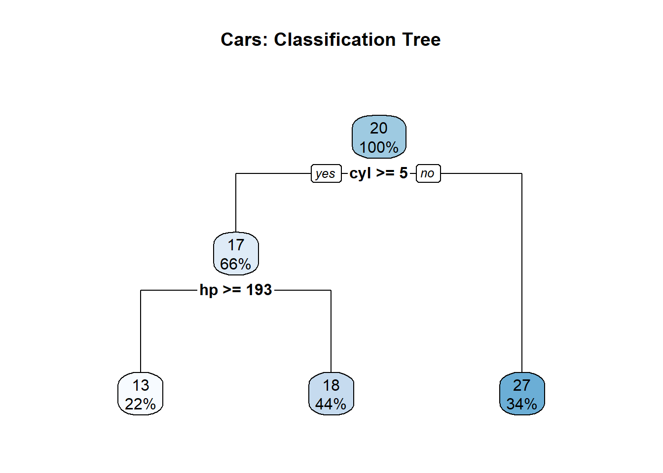
# Passing in a `type=1,2,3,4, or 5` value changes the appearance of the tree
rpart.plot(tree_model, main = 'Cars: Classification Tree', type=2)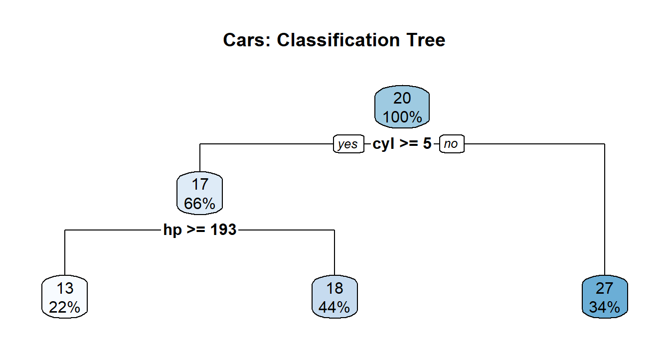
Basic Modeling with Cross-Validation in R
We use cross-validation as a “a statistical approach for determining how well the results of a statistical investigation generalize to a different data set” (finnstats, 2021). The library(caret) will help us in this endeavor.
Train Test Split
set.seed(222) # for reproducibility
dt <- sort(sample(nrow(mtcars), nrow(mtcars)*.75))
train_cars <-mtcars[dt,]
test_cars <-mtcars[-dt,]

# check size dimensions of respective partitions
n_train <- nrow(train_cars)[1]
n_test <- nrow(test_cars)[1]

train_size = n_train/(n_train+n_test)
test_size = n_test/(n_train+n_test)

cat('\n Train Size:', train_size,
    '\n Test Size:', test_size)
##
## Train Size: 0.75
## Test Size: 0.25Let us bring in a generalized linear model for this illustration.
cars_model <- glm(mpg ~., data = mtcars)
cars_predictions <- predict(cars_model, test_cars)

# computing model performance metrics
data.frame(R2 = R2(cars_predictions, test_cars$mpg),
           RMSE = RMSE(cars_predictions, test_cars$mpg),
           MAE = MAE(cars_predictions, test_cars$mpg))
## R2 RMSE MAE
## 1 0.9149732 1.72719 1.400446In order to use the trainControl() function for cross-validation, we will bring in the library(caret).
library(caret)# Best model has lowest error(s)
# Now let us train the model with cross-validation
train_control <- trainControl(method = "cv", number = 5, savePredictions=TRUE)
cars_predictions <- train(mpg ~., data=mtcars, # glm model
method = 'glm',
trControl = train_control) # cross-validation
cars_predictions## Generalized Linear Model
##
## 32 samples
## 10 predictors
##
## No pre-processing
## Resampling: Cross-Validated (5 fold)
## Summary of sample sizes: 24, 26, 25, 26, 27
## Resampling results:
##
## RMSE Rsquared MAE
## 3.12627 0.8167969 2.587204K-Means Clustering
A cluster is a collection of observations. We want to group these observations based on the most similar attributes. We use distance measures to measure similarity between clusters.
This is one of the most widely-used unsupervised learning techniques that groups “similar data points together and discover underlying patterns. To achieve this objective, K-means looks for a fixed number (k) of clusters in a dataset” (Garbade, 2018).
# Let us split the mtcars dataset into 3 clusters.
library(cluster)    # clustering algorithms
library(factoextra) # clustering algorithms & visualization
## Welcome! Want to learn more? See two factoextra-related books at https://goo.gl/ve3WBaset.seed(222)
kmeans_cars <- kmeans(mtcars, # dataset
centers = 3, # number of centroids
nstart = 20) # number of random starts s/b > 1
kmeans_cars ## K-means clustering with 3 clusters of sizes 16, 7, 9
##
## Cluster means:
## mpg cyl disp hp drat wt
## 1 24.50000 4.625000 122.2937 96.8750 4.002500 2.518000
## 2 17.01429 7.428571 276.0571 150.7143 2.994286 3.601429
## 3 14.64444 8.000000 388.2222 232.1111 3.343333 4.161556
## qsec vs am gear carb
## 1 18.54312 0.7500000 0.6875000 4.125000 2.437500
## 2 18.11857 0.2857143 0.0000000 3.000000 2.142857
## 3 16.40444 0.0000000 0.2222222 3.444444 4.000000
##
## Clustering vector:
## Mazda RX4 Mazda RX4 Wag Datsun 710
## 1 1 1
## Hornet 4 Drive Hornet Sportabout Valiant
## 2 3 2
## Duster 360 Merc 240D Merc 230
## 3 1 1
## Merc 280 Merc 280C Merc 450SE
## 1 1 2
## Merc 450SL Merc 450SLC Cadillac Fleetwood
## 2 2 3
## Lincoln Continental Chrysler Imperial Fiat 128
## 3 3 1
## Honda Civic Toyota Corolla Toyota Corona
## 1 1 1
## Dodge Challenger AMC Javelin Camaro Z28
## 2 2 3
## Pontiac Firebird Fiat X1-9 Porsche 914-2
## 3 1 1
## Lotus Europa Ford Pantera L Ferrari Dino
## 1 3 1
## Maserati Bora Volvo 142E
## 3 1
##
## Within cluster sum of squares by cluster:
## [1] 32838.00 11846.09 46659.32
## (between_SS / total_SS = 85.3 %)
##
## Available components:
##
## [1] "cluster" "centers" "totss"
## [4] "withinss" "tot.withinss" "betweenss"
## [7] "size" "iter" "ifault"
Now let’s visualize the cluster using the fviz_cluster() function from the factoextra library.
fviz_cluster(kmeans_cars,
             data = mtcars) +
theme_classic() 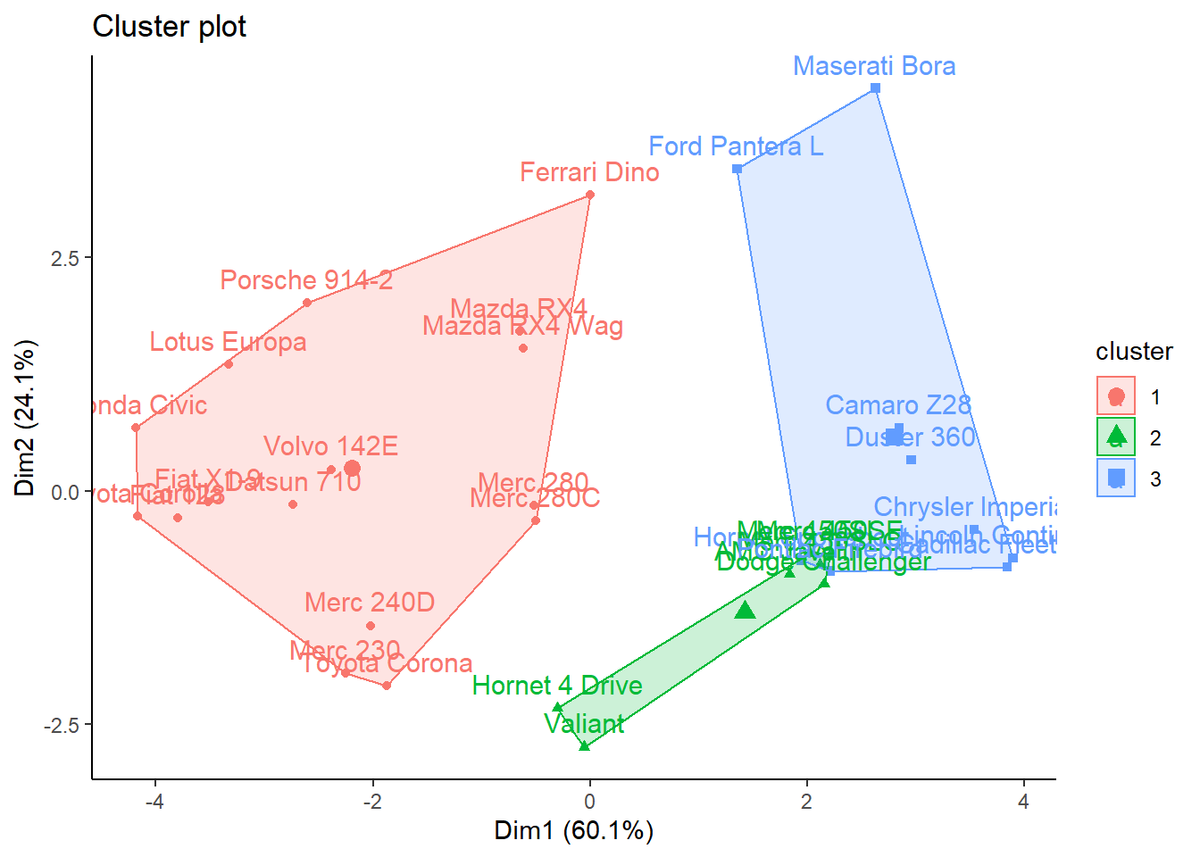
But what is the appropriate number of clusters that we should generate? Can we do better with more clusters?
# total sum of squares
kmeans_cars$totss
## [1] 623387.5# between sum of squares
kmeans_cars$betweenss## [1] 532044.1# within sum of squares
kmeans_cars$withinss ## [1] 32838.00 11846.09 46659.32# ratio for between sum of squares/ total sum of squares
kmeans_cars$betweenss/kmeans_cars$totss ## [1] 0.8534725Let’s create a numeric vector populated with zeroes and ten spots long.
wss <- numeric(10)Can we do better? Let’s run k-means from 1:10 clusters.
This will effectively measure the homogeneity of the clusters as the number of clusters increases.
Now let us use a basic for-loop to run through k-means 10 times. K-means is iterated through each of these 10 clusters as follows:
# using within sum of squares

for(i in 1:10) {
  wss[i] <- sum(kmeans
               (mtcars,
                centers=i)
                $withinss)
}
Basic Elbow Method
Now let’s plot these within sum of squares using the elbow method, which is one of the most commonly used approaches for finding the optimal k.
plot(wss,
     type='b',
     main ='Elbow Method for K-Means',
col='blue') 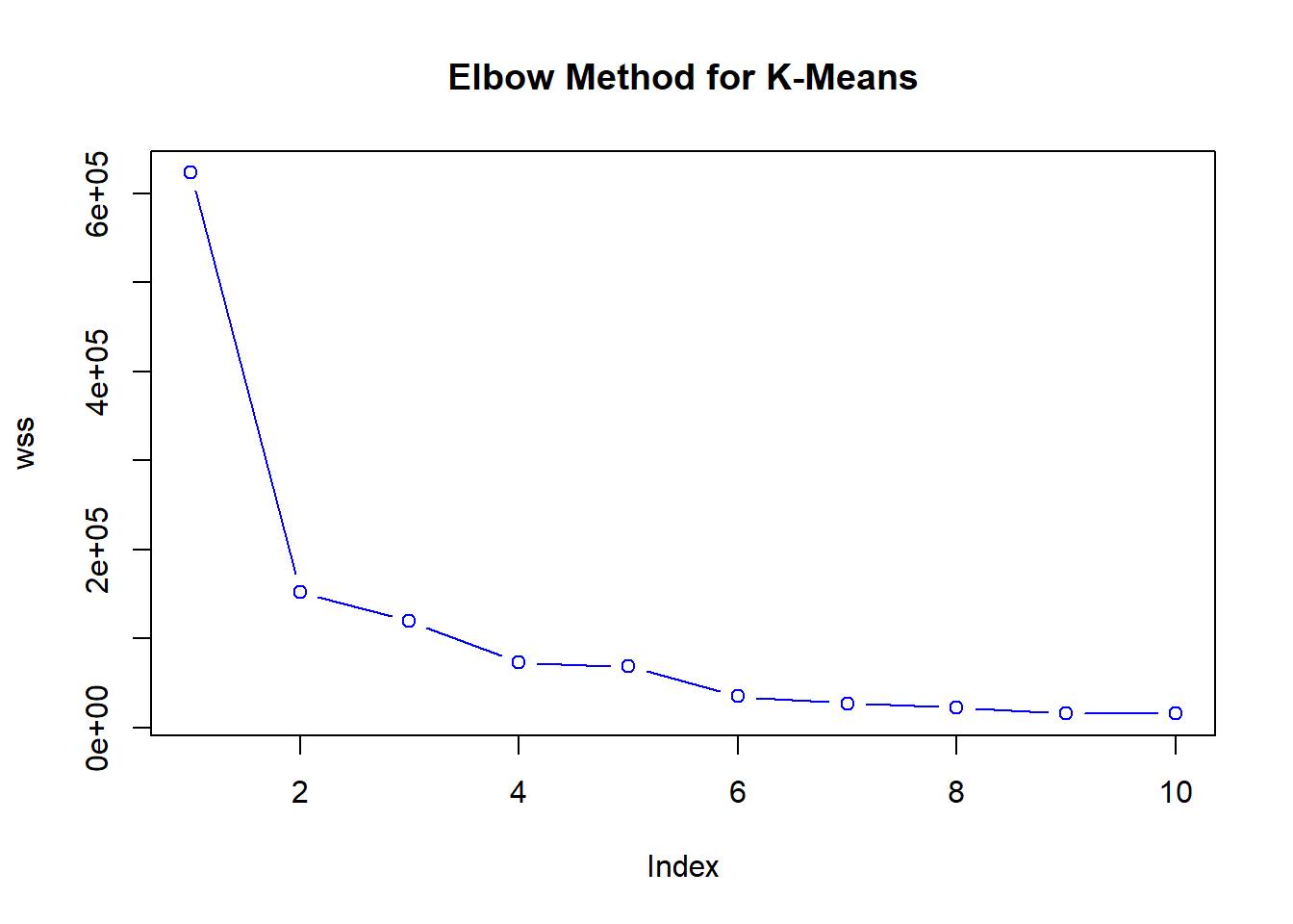
Once we start to add clusters, the within sum of squares is reduced. Thus, the incremental reduction in within sum of squares is getting progressively smaller. We see that after approximately k = 3, each of the new clusters is not separating the data as well.
Hierarchical Clustering
This is another form of unsupervised learning type of cluster analysis, which takes on a more visual method, working particularly well with smaller samples (i.e., n < 500), such as this mtcars dataset. We start out with as many clusters as observations, and we go through a procedure of combining observations into clusters, and culminating with combining clusters together as a reduction method for the total number of clusters that are present. Moreover, the premise for combining clusters together is a direct result of:
complete linkage - or largest Euclidean distance between clusters.
single linkage - conversely, we look at the observations which are closest together (proximity).
centroid linkage - we can the distance between the centroid of each cluster.
group average (mean) linkage - taking the mean between the pairwise distances of the observations.
Complete linkage is the most traditional approach.
The tree structure that examines this hierarchical structure is called a dendogram.
auto_dist <- dist(mtcars,
                  method ='euclidean',
                  diag = FALSE)

auto_cluster <- hclust(auto_dist,
                       method ='complete')
# plot the hierarchical cluster
plot(auto_cluster)
rect.hclust(auto_cluster, k = 3, border = 'red') # visualize cluster borders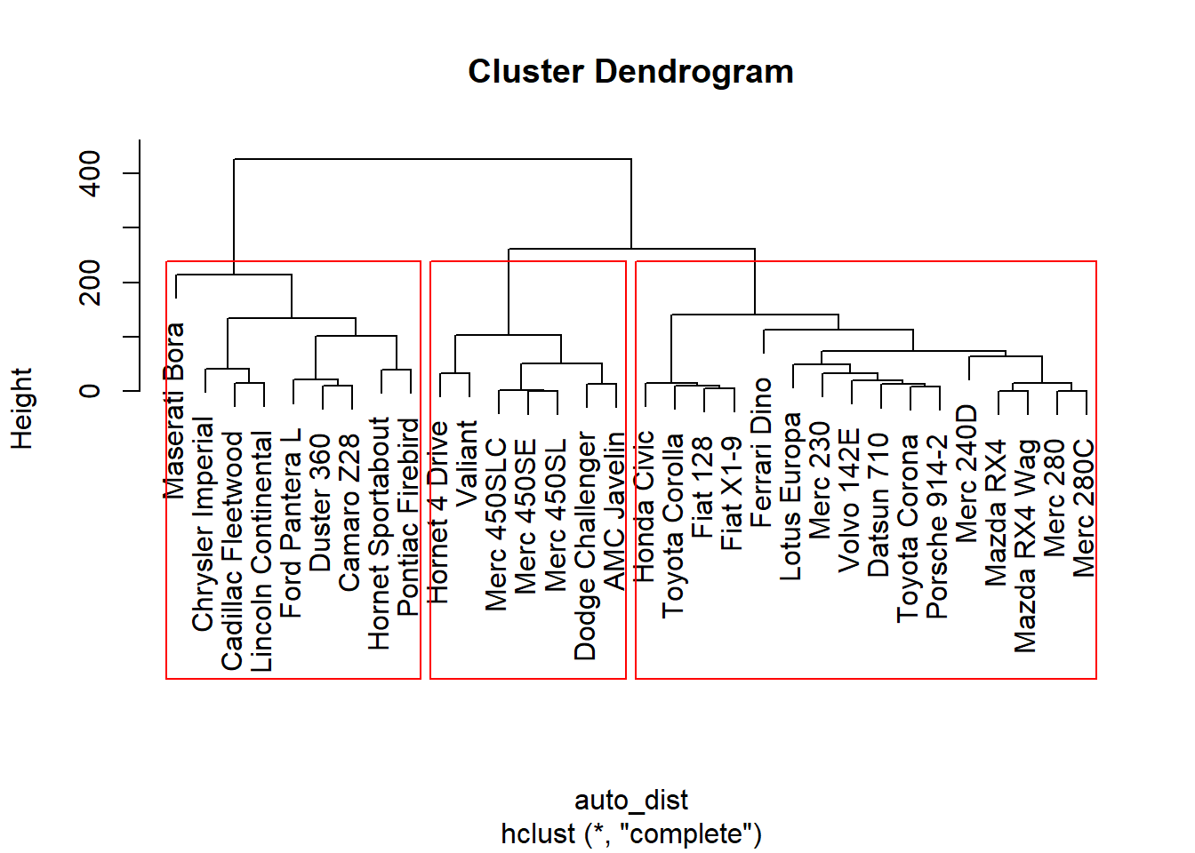
Our dendogram indicates which observation is within which cluster.
We can cut our tree at let’s say 3 clusters, segmenting them out as follows:
cut_tree <- cutree(auto_cluster, 3) # each obs. now belongs to cluster 1,2, or 3
mtcars$segment <- cut_tree # segment out the data
Now we can view our segmented data in the workspace window as follows:
View(mtcars)Or see it as a dataframe, per usual:
print(mtcars)## mpg cyl disp hp drat wt qsec vs
## Mazda RX4 21.0 6 160.0 110 3.90 2.620 16.46 0
## Mazda RX4 Wag 21.0 6 160.0 110 3.90 2.875 17.02 0
## Datsun 710 22.8 4 108.0 93 3.85 2.320 18.61 1
## Hornet 4 Drive 21.4 6 258.0 110 3.08 3.215 19.44 1
## Hornet Sportabout 18.7 8 360.0 175 3.15 3.440 17.02 0
## Valiant 18.1 6 225.0 105 2.76 3.460 20.22 1
## Duster 360 14.3 8 360.0 245 3.21 3.570 15.84 0
## Merc 240D 24.4 4 146.7 62 3.69 3.190 20.00 1
## Merc 230 22.8 4 140.8 95 3.92 3.150 22.90 1
## Merc 280 19.2 6 167.6 123 3.92 3.440 18.30 1
## Merc 280C 17.8 6 167.6 123 3.92 3.440 18.90 1
## Merc 450SE 16.4 8 275.8 180 3.07 4.070 17.40 0
## Merc 450SL 17.3 8 275.8 180 3.07 3.730 17.60 0
## Merc 450SLC 15.2 8 275.8 180 3.07 3.780 18.00 0
## Cadillac Fleetwood 10.4 8 472.0 205 2.93 5.250 17.98 0
## Lincoln Continental 10.4 8 460.0 215 3.00 5.424 17.82 0
## Chrysler Imperial 14.7 8 440.0 230 3.23 5.345 17.42 0
## Fiat 128 32.4 4 78.7 66 4.08 2.200 19.47 1
## Honda Civic 30.4 4 75.7 52 4.93 1.615 18.52 1
## Toyota Corolla 33.9 4 71.1 65 4.22 1.835 19.90 1
## Toyota Corona 21.5 4 120.1 97 3.70 2.465 20.01 1
## Dodge Challenger 15.5 8 318.0 150 2.76 3.520 16.87 0
## AMC Javelin 15.2 8 304.0 150 3.15 3.435 17.30 0
## Camaro Z28 13.3 8 350.0 245 3.73 3.840 15.41 0
## Pontiac Firebird 19.2 8 400.0 175 3.08 3.845 17.05 0
## Fiat X1-9 27.3 4 79.0 66 4.08 1.935 18.90 1
## Porsche 914-2 26.0 4 120.3 91 4.43 2.140 16.70 0
## Lotus Europa 30.4 4 95.1 113 3.77 1.513 16.90 1
## Ford Pantera L 15.8 8 351.0 264 4.22 3.170 14.50 0
## Ferrari Dino 19.7 6 145.0 175 3.62 2.770 15.50 0
## Maserati Bora 15.0 8 301.0 335 3.54 3.570 14.60 0
## Volvo 142E 21.4 4 121.0 109 4.11 2.780 18.60 1
## am gear carb segment
## Mazda RX4 1 4 4 1
## Mazda RX4 Wag 1 4 4 1
## Datsun 710 1 4 1 1
## Hornet 4 Drive 0 3 1 2
## Hornet Sportabout 0 3 2 3
## Valiant 0 3 1 2
## Duster 360 0 3 4 3
## Merc 240D 0 4 2 1
## Merc 230 0 4 2 1
## Merc 280 0 4 4 1
## Merc 280C 0 4 4 1
## Merc 450SE 0 3 3 2
## Merc 450SL 0 3 3 2
## Merc 450SLC 0 3 3 2
## Cadillac Fleetwood 0 3 4 3
## Lincoln Continental 0 3 4 3
## Chrysler Imperial 0 3 4 3
## Fiat 128 1 4 1 1
## Honda Civic 1 4 2 1
## Toyota Corolla 1 4 1 1
## Toyota Corona 0 3 1 1
## Dodge Challenger 0 3 2 2
## AMC Javelin 0 3 2 2
## Camaro Z28 0 3 4 3
## Pontiac Firebird 0 3 2 3
## Fiat X1-9 1 4 1 1
## Porsche 914-2 1 5 2 1
## Lotus Europa 1 5 2 1
## Ford Pantera L 1 5 4 3
## Ferrari Dino 1 5 6 1
## Maserati Bora 1 5 8 3
## Volvo 142E 1 4 2 1Sources
finnstats. (2021, October 31). What Does Cross Validation Mean? R-bloggers.Garbade, Michael. (2018, September 12). Understanding K-means Clustering in
-
Machine Learning. Towards Data Science.
https://towardsdatascience.com/understanding-k-means-clustering-in-machine-learning-6a6e67336aa1
Shmueli, G., Bruce, P. C., Yahav, I., Patel, N. R., & Lichtendahl Jr., K. C. (2018).
-
Data mining for business analytics: Concepts, techniques, and applications in R. Wiley.