['Birthday',
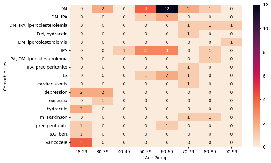
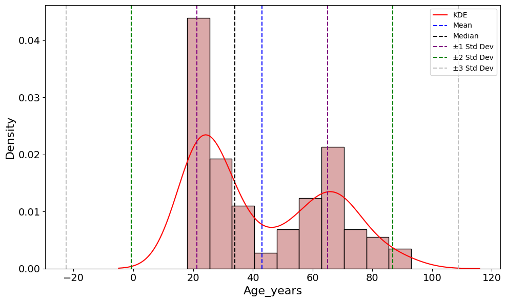
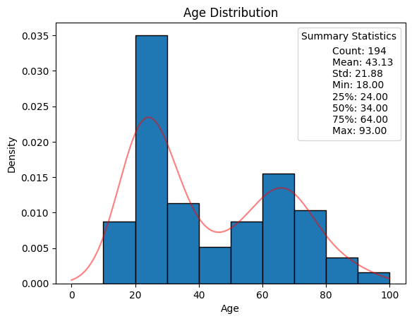
'Age_years',
'Weight_kg',
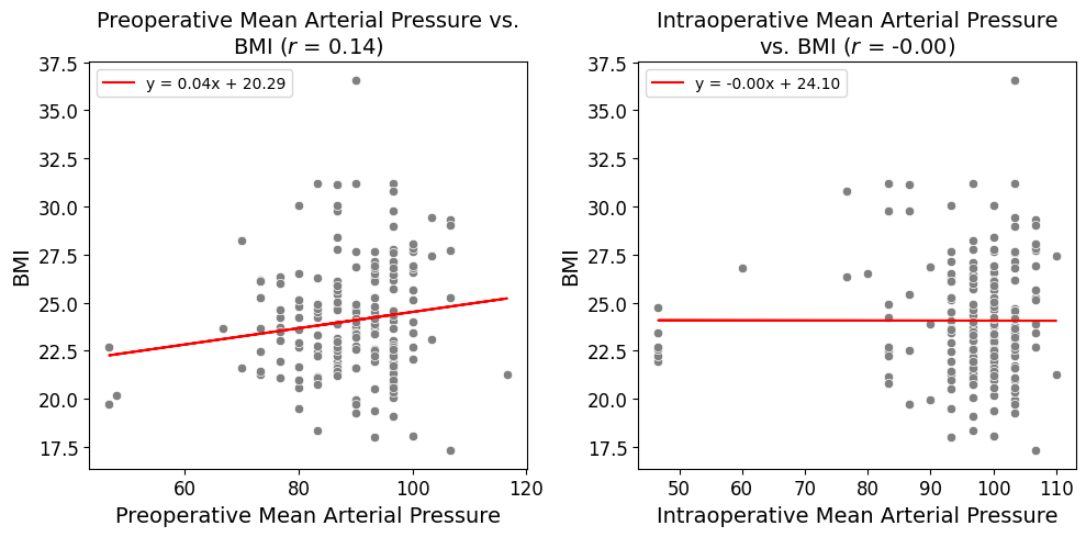
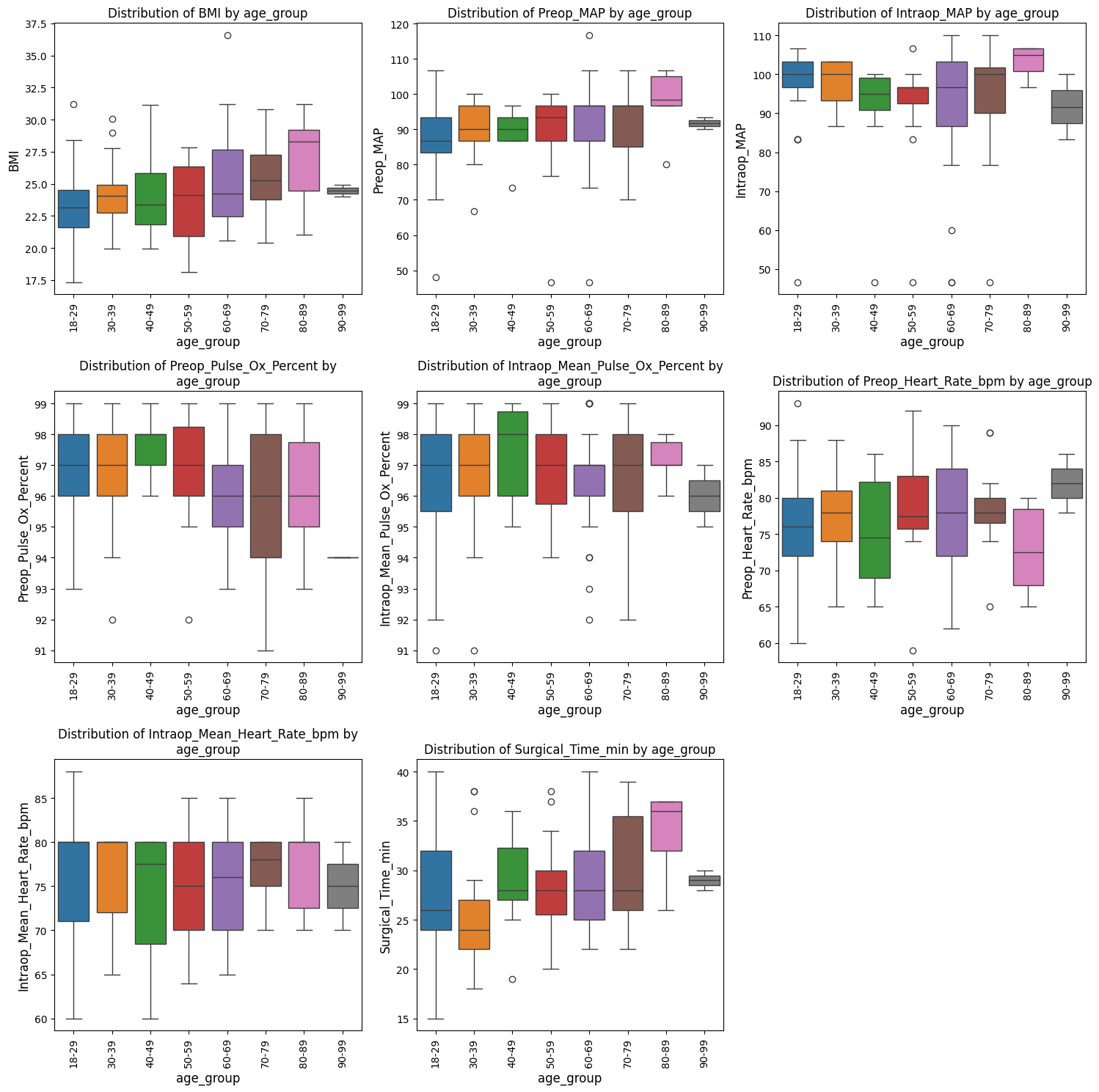
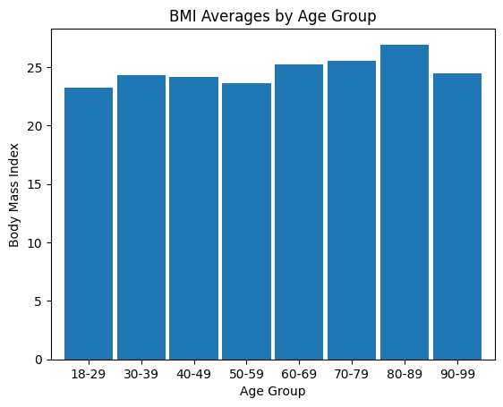
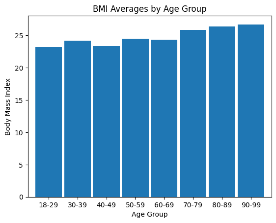
'BMI',
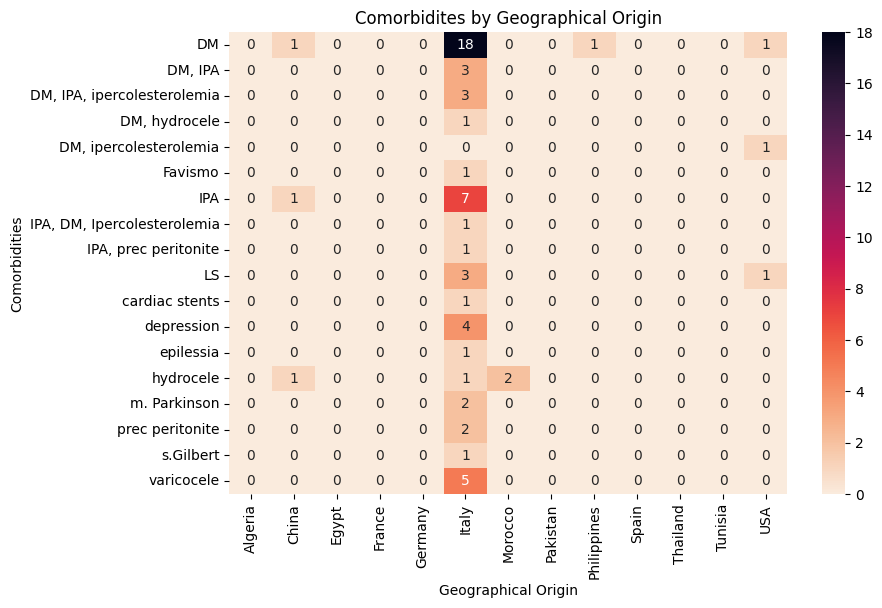
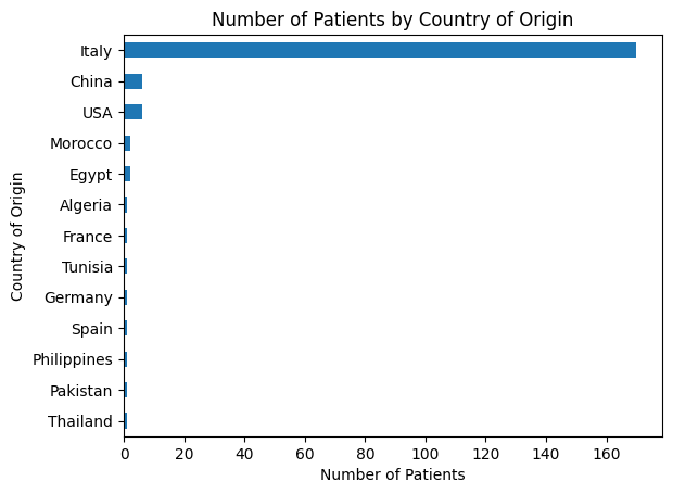
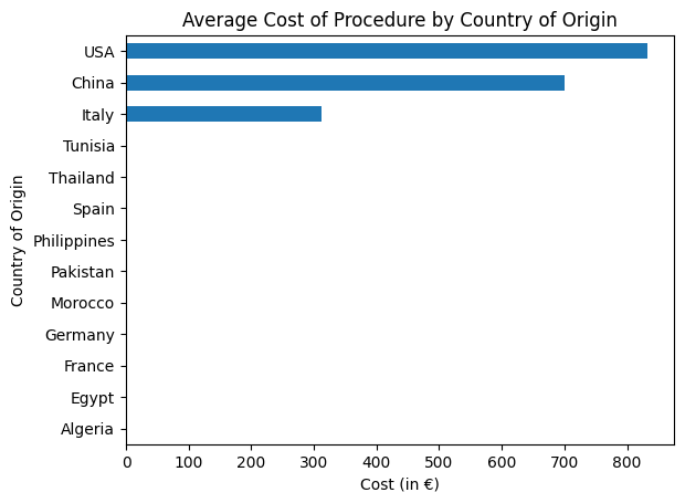
'Geographical_Origin',
'Cultural_Religious_Affiliation',
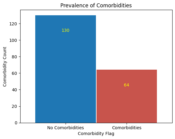
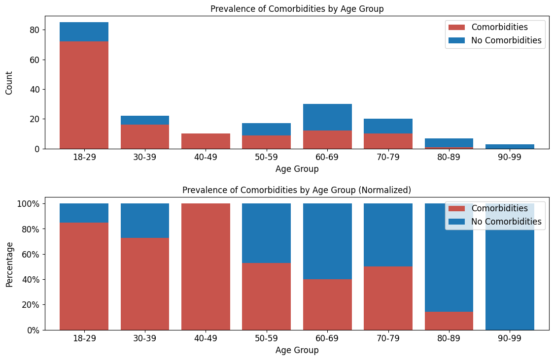
'Comorbidities',
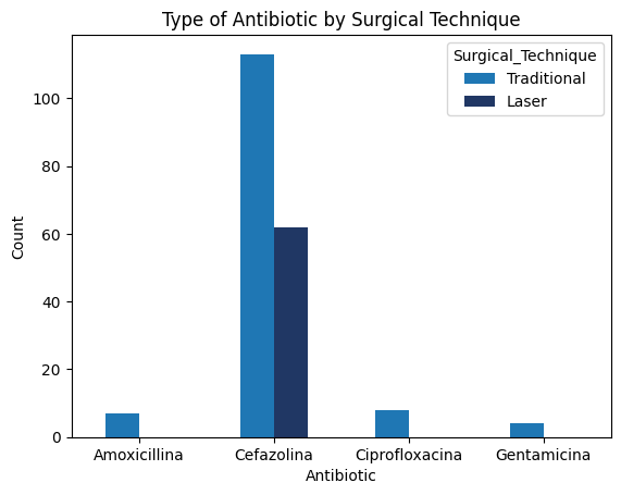
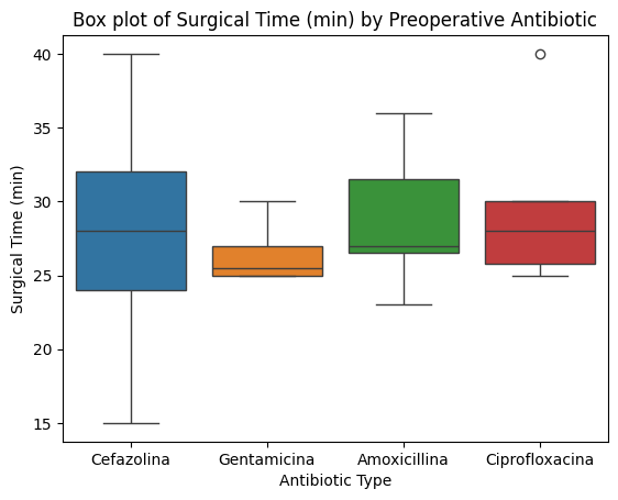
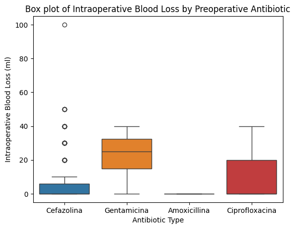
'Preop_drugs_antibiotic',
'Preop_Blood_Pressure_mmHg',
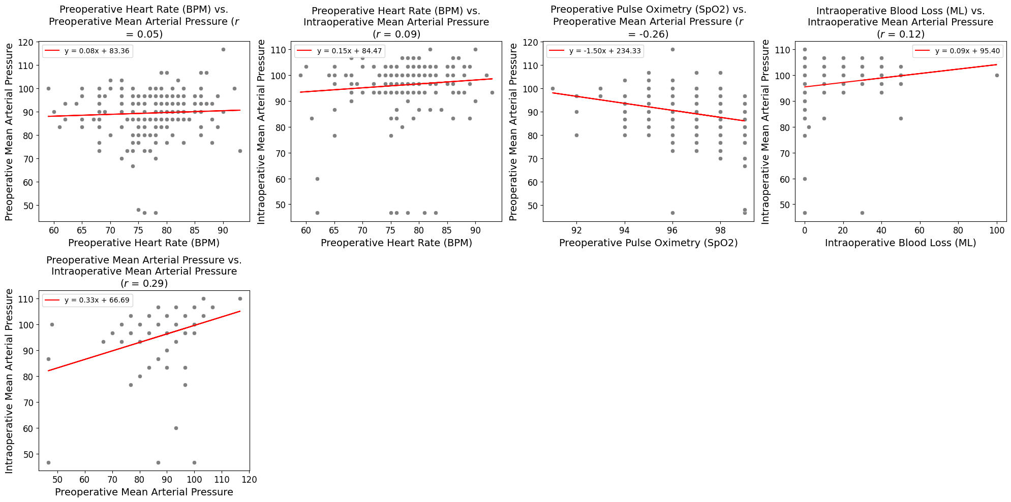
'Preop_Heart_Rate_bpm',
'Preop_Pulse_Ox_Percent',
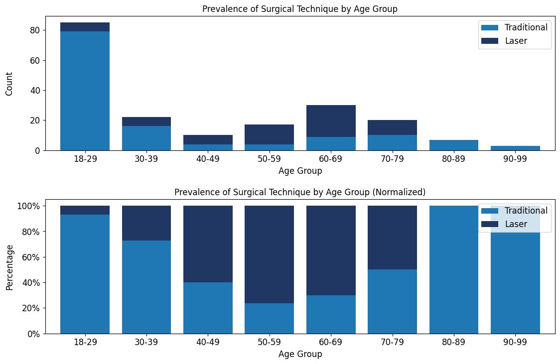
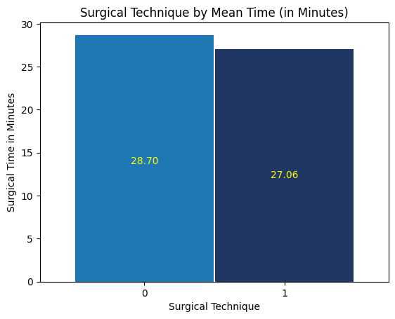
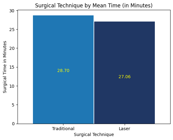
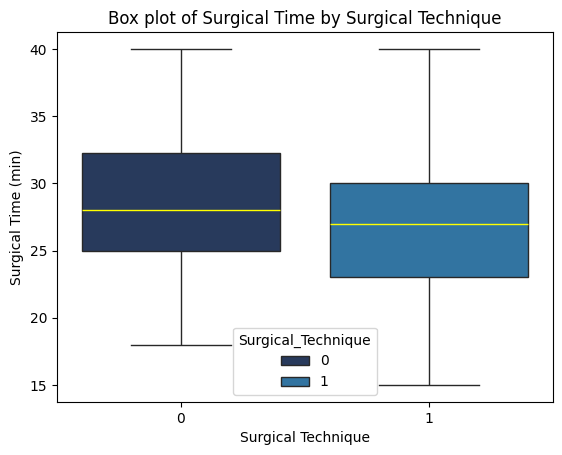
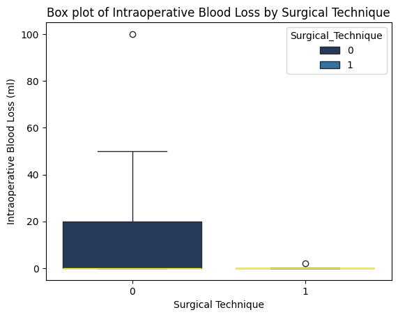
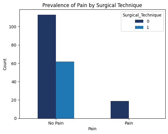
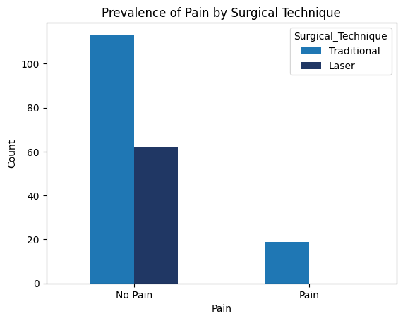
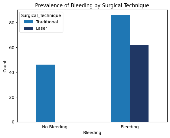
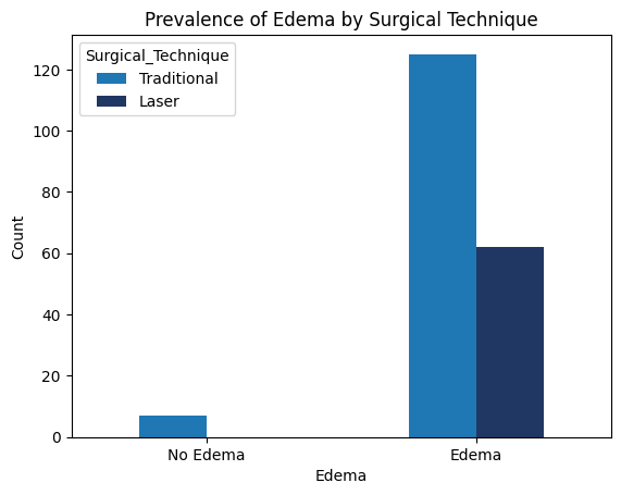
'Surgical_Technique',
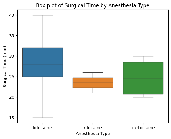
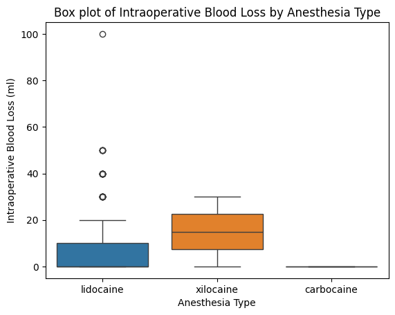
'Anesthesia_Type',
'Intraoperative_drugs',
'Intraoperative_Blood_Loss_ml',
'Intraop_Mean_Blood_Pressure_mmHg',
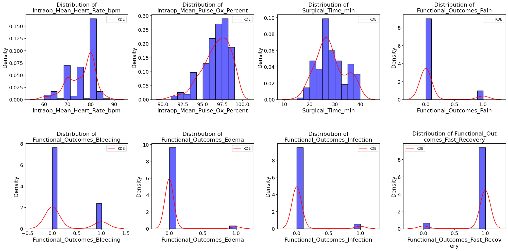
'Intraop_Mean_Heart_Rate_bpm',
'Intraop_Mean_Pulse_Ox_Percent',
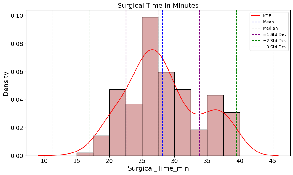
'Surgical_Time_min',
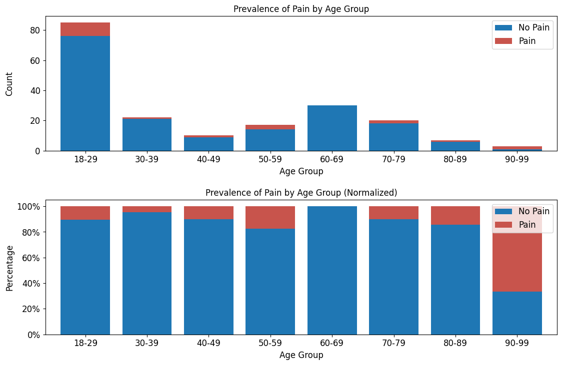
'Functional_Outcomes_Pain',
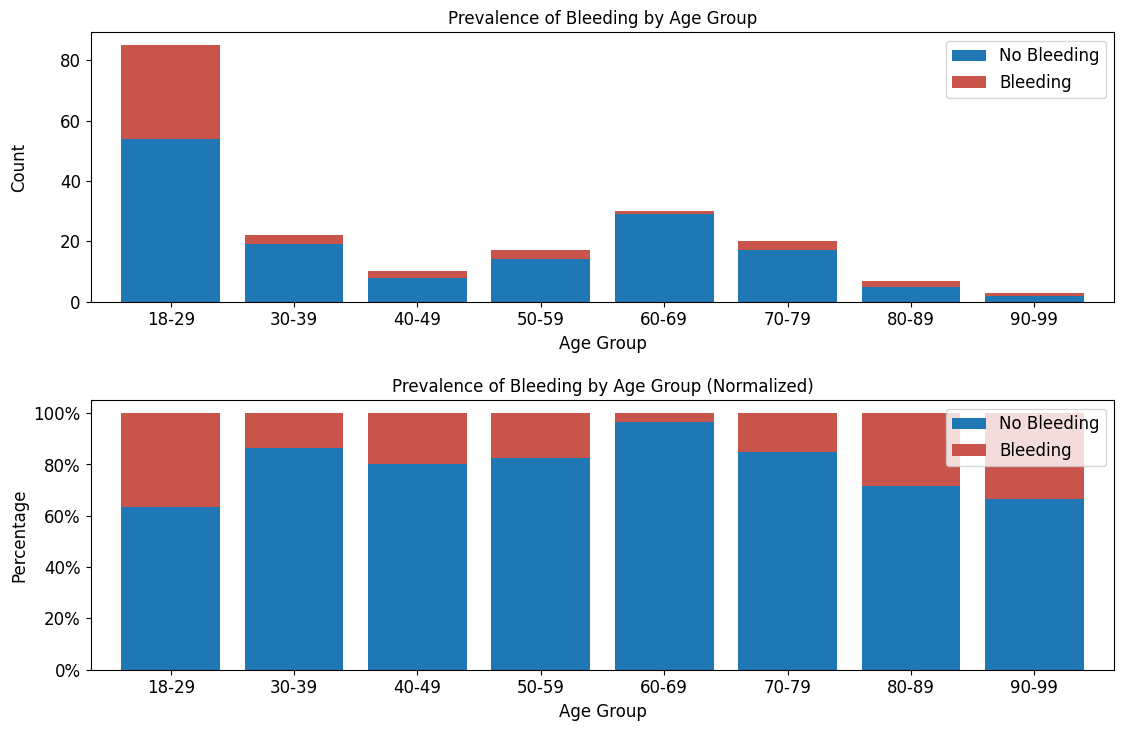
'Functional_Outcomes_Bleeding',
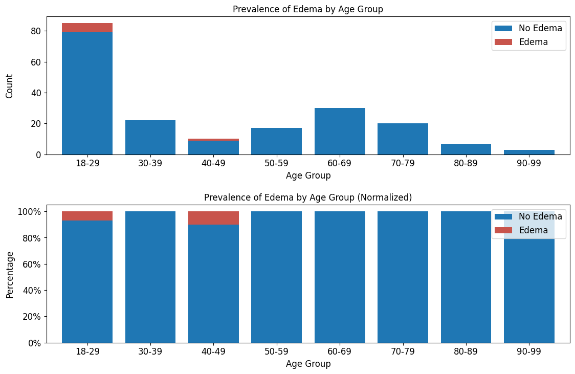
'Functional_Outcomes_Edema',
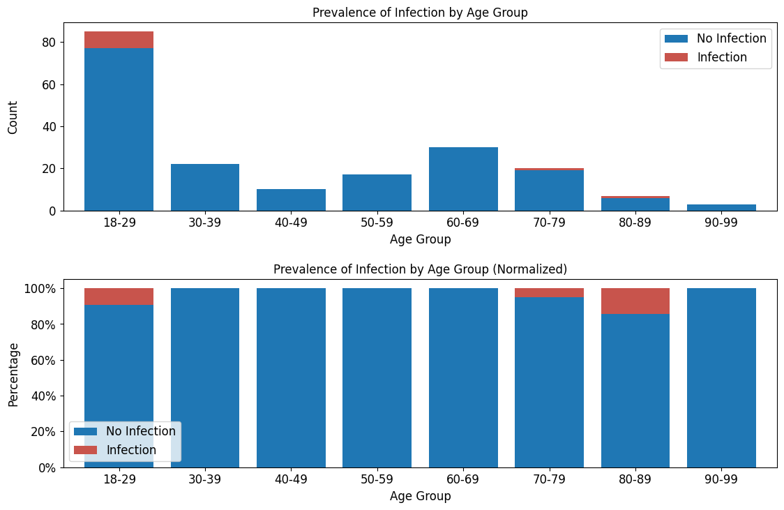
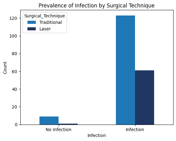
'Functional_Outcomes_Infection',
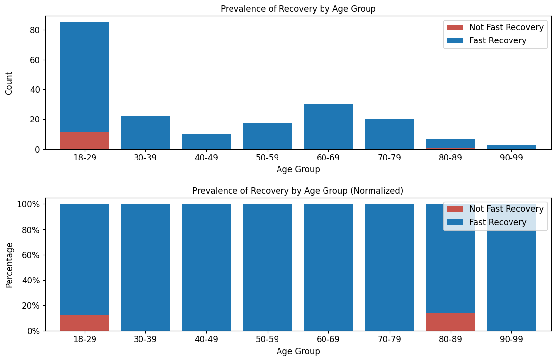
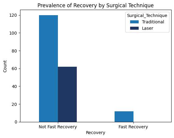
'Functional_Outcomes_Fast_Recovery',
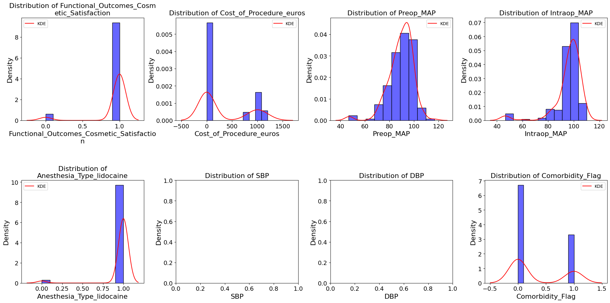
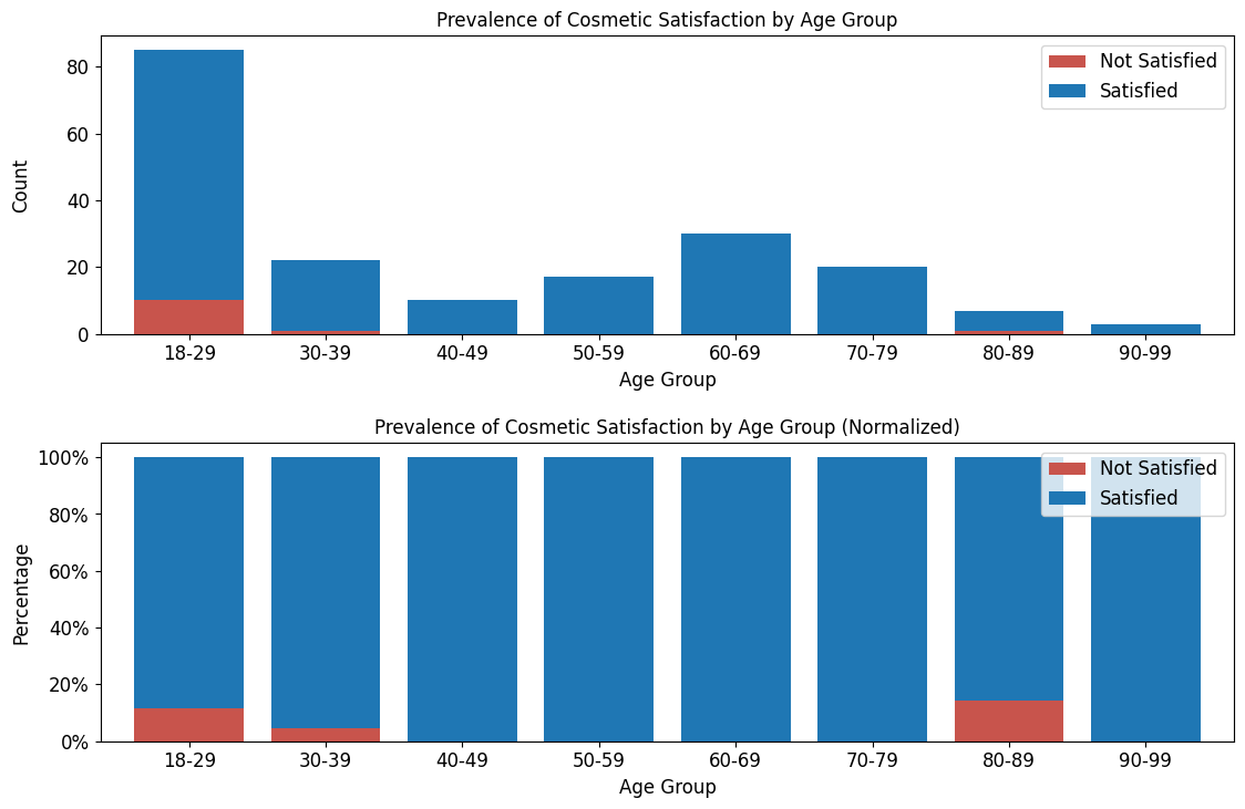
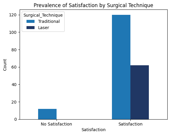
'Functional_Outcomes_Cosmetic_Satisfaction',
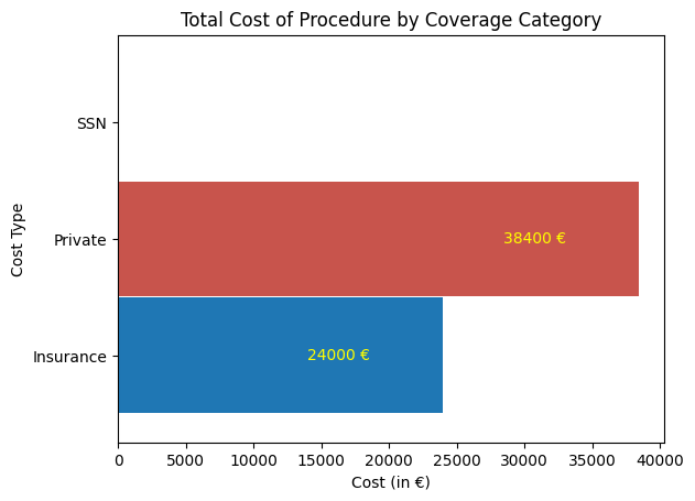
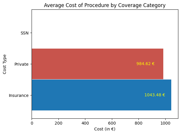
'Cost_of_Procedure_euros',
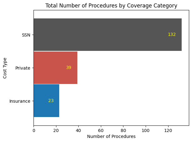
'Cost_Type',
'BMI_Category',
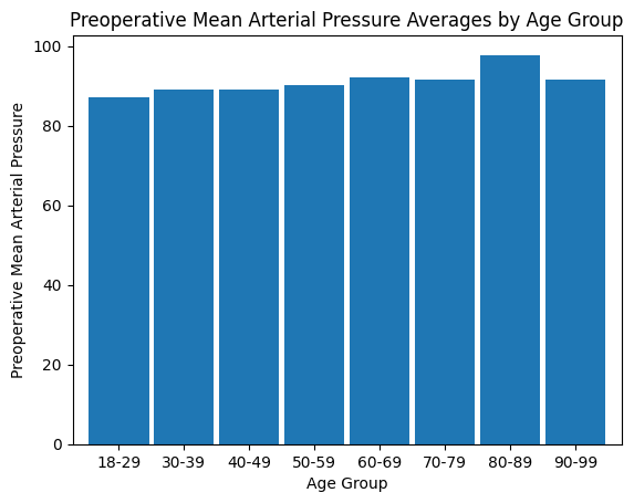
'Preop_MAP',
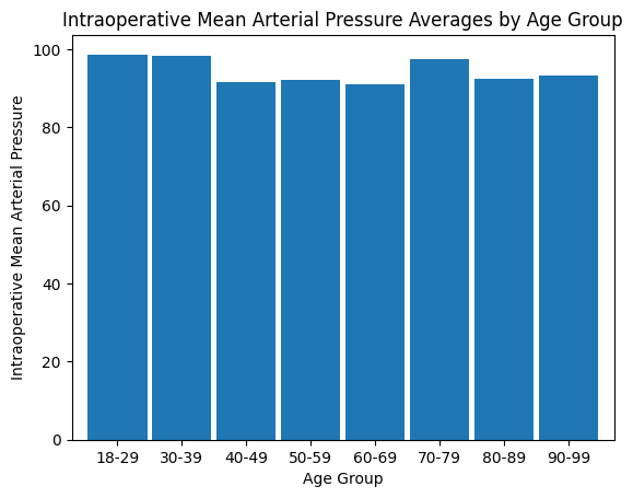
'Intraop_MAP',
'Diabetes',
'Anesthesia_Type_carbocaine',
'Anesthesia_Type_lidocaine',
'BMI_Category_Normal_Weight',
'BMI_Category_Obese',
'BMI_Category_Overweight',
'BMI_Category_Underweight',
'Intraop_SBP',
'Intraop_DBP',
'Preop_SBP',
'Preop_DBP',
'Comorbidity_Flag']