Python Introductory Workshop by University of San Diego (USD)
Leonid Shpaner
January 21, 2022
Whereas JupyterLab and Jupyter Notebook are the two most commonly used interactive computing platforms warehoused within the Anaconda distribution, data scientists can also leverage the cloud-based coding environment of Google Colab.
JupyterLab Basics
https://jupyterlab.readthedocs.io/en/stable/user/interface.html
Cells
# This is a code cell/block!

# basic for loop
for x in [1,2,3]:
    print(x)
This is a markdown cell!
Level 3 Heading
italics characters are surrounded by one asterisk
bold characters are surrounded by two asterisks
- one asterisk in front of an item of text can serve as a bullet point.
- to move the text to the next line, ensure to enter two spaces after the line.
- Simply number the items on a list using normal numering schema.
- If you have numbers in the same markdown cell as bullet points (i.e., below),
- skip 4 spaces after the last bullet point and then begin numbering.
Here's a guide for syntax: https://www.markdownguide.org/basic-syntax/
Python Basics
We can use a code cell to conduct basic math operations as follows.
2+2
Order of operations in Python is just as important.
1+3*10 == (1+3)*10
For more basic operations including but not limited to taking the square root, log, and generally more advanced mathematical operations, we will have to import our first library (math) as follows:
import math
However, if we run two consecutive lines below without assigning to a variable or parsing in a print statement ahead of the function calls, only the latest (last) function will print the output of what is in the cell block.
math.sqrt(9)
math.log10(100)
math.factorial(10)
Let us try this again, by adding print() statements in front of the three functions, respectively.
# print the output on multiple lines
print(math.sqrt(9))
print(math.log10(100))
print(math.factorial(10))
What is a string?
A string is simply any open alpha/alphanumeric text characters surrounded by either single quotation marks or double quotation marks, with no preference assigned for either single or double quotation marks, with a print statement being called prior to the strings. For example,
print('This is a string.')
print( "This is also a string123.")
Strings in Python are arrays of bytes that represent "Unicode characters" (GeeksforGeeks, 2021).
Creating Objects
Unlike R, Python uses the '=' symbol for making assignment statements. we can print() what is contained in the assignment or just call the assignment to the string as follows:
cheese = 'pepper jack'
cheese
Determining and Setting the Current Working Directory
The importance of determining and setting the working directory cannot be stressed enough.
- Run
import osto import operating system module. - then assign
os.getcwd()tocwd. - You may choose to print the working directory using the print function as shown below.
- Or change the working directory by running
os.chdir('').
import os # import the operating system module
cwd = os.getcwd()
# Print the current working directory
print("Current working directory: {0}".format(cwd))

# Change the current working directory
# os.chdir('')

# Print the current working directory
print("Current working directory: {0}".format(os.getcwd()))
Installing Libraries
To install most common libraries, simply type in the command pip install followed by library name into an empty code cell and run it.
# pip install pandas
Loading Libraries
For data science applications, we most commonly use pandas for "data structures and data analysis tools" (Pandas, 2021) and NumPy for "scientific computing with Python" (Numpy.org, n.d.).
Ideally, at the beginning of a project, we will create an empty cell block that loads all of the libraries that we will be using. However, as we progress throughout this tutorial, we will load the necessary libraries separately.
Let us now load these two libraries into an empty code cell block using import name of the library as abbreviated form.
import pandas as pd
import numpy as np
Sometimes, Python throws warning messages in pink on the output of code cell blocks that otherwise run correctly.
import warnings
warnings.warn('This is an example warning message.') # displaying warning
Sometimes, it is helpful to see what these warnings are saying as added layers of de-bugging. However, they may also create unsightly output. For this reason, we will suppress any and all warning messages for the remainder of this tutorial.
To disable/suppress warning messages, let us write the following:
import warnings
warnings.filterwarnings("ignore")
Data Types
Text Type (string): str
Numeric Types: int, float, complex
Sequence Types: list, tuple, range
Mapping Type: dict - dictionary (used to store key:value pairs)
Logical: bool - boolean (True or False)
Binary Types: bytes, bytearray, memoryview
Let us convert an integer to a string. We do this using the str() function. Recall, how in R, this same function call is designated for something completely different - inspecting the structure of the dataframe.
We can also examine floats and bools as follows:
# assign the variable to an int
int_numb  = 2356
print('Integer:', int_numb)

# assign the variable to a float
float_number = 2356.0
print('Float:', float_number)

# convert the variable to a string
str_numb = str(int_numb)
print('String:',str_numb)

# convert variable from float to int
int_number = int(float_number)

# boolean
bool1 = 2356 > 235
bool2 = 2356 == 235
print(bool1)
print(bool2)
Data Structures
What is a variable? A variable is a container for storing a data value, exhibited as a reference to "to an object in memory which means that whenever a variable is assigned to an instance, it gets mapped to that instance. A variable in R can store a vector, a group of vectors or a combination of many R objects" (GeeksforGeeks, 2020).
There are 3 most important data structures in Python: vector, matrix, and dataframe.
Vector: the most basic type of data structure within R; contains a series of values of the same data class. It is a "sequence of data elements" (Thakur, 2018).
Matrix: a 2-dimensional version of a vector. Instead of only having a single row/list of data, we have rows and columns of data of the same data class.
Dataframe: the most important data structure for data science. Think of dataframe as loads of vectors pasted together as columns. Columns in a dataframe can be of different data class, but values within the same column must be the same data class.
Creating Objects
We can make a one-dimensional horizontal list as follows:
list1 = [0, 1, 2, 3]
list1
or a one-dimensional vertical list as follows:
list2 = [[1],
         [2],
         [3],
         [4]]
list2
Vectors and Their Operations
Now, to vectorize these lists, we simply assign it to the np.array() function call:
vector1 = np.array(list1)
print(vector1)
print('\n') # for printing an empty new line
            # between outputs
vector2 = np.array(list2)
print(vector2)
Running the following basic between vector arithmetic operations (addition, subtraction, and division, respectively) changes the resulting data structures from one-dimensional arrays to two-dimensional matrices.
# adding vector 1 and vector 2
addition = vector1 + vector2

# subtracting vector 1 and vector 2
subtraction = vector1 - vector2

# multiplying vector 1 and vector 2
multiplication = vector1 * vector2

# divifing vector 1 by vector 2
division = vector1 / vector2

# Now let's print the results of these operations
print('Vector Addition: ', '\n', addition, '\n')
print('Vector Subtraction:', '\n', subtraction, '\n')
print('Vector Multiplication:', '\n', multiplication, '\n')
print('Vector Division:', '\n', division)
Similarly, a vector of logical strings will contain
vector3 = np.array([True, False, True, False, True])
vector3
Whereas in R, we use the length() function to measure the length of an object (i.e., vector, variable, or dataframe), we apply the len() function in Python to determine the number of members inside this object.
len(vector3)
Let us say for example, that we want to access the third element of vector1 from what we defined above. In this case, the syntax is the same as in R. We can do so as follows:
vector1[3]
Let us now say we want to access the first, fifth, and ninth elements of this dataframe. To this end, we do the following:
vector4 = np.array([1,3,5,7,9,20,2,8,10,35,76,89,207])
vector4_index = vector4[1], vector4[5], vector4[9]
vector4_index
What if we wish to access the third element on the first row of this matrix?
# create (define) new matrix
matrix1 = np.array([[1,2,3,4,5], [6,7,8,9,10],
                [11,12,13,14,15]])
print(matrix1)

print('\n','3rd element on 1st row:', matrix1[0,2])
Counting Numbers and Accessing Elements in Python
Whereas it would make sense to start counting items in an array with the number 1 like we do in R, this is not true in Python. We ALWAYS start counting items with the number 0 as the first number of any given array in Python.
What if we want to access certain elements within the dataframe? For example:
# find the length of vector 1
print(len(vector1))

# get all elements
print(vector1[0:4])

# get all elements except last one
print(vector1[0:3])
Mock Dataframe Examples
Unlike R, creating a dataframe in Python involves a little bit more work. For example, we will be using the pandas library to create what is called a pandas dataframe using the pd.DataFrame() function and map our variables to a dictionary. Like we previously discussed, a dictionary is used to index key:value pairs and to store these mapped values. Dictionaries are always started (created) using the { symbol, followed by the name in quotation marks, a :, and an opening [. They are ended using the opposite closing symbols.
Let us create a mock dataframe for five fictitious individuals representing different ages, and departments at a research facility.
df = pd.DataFrame({'Name': ['Jack', 'Kathy', 'Latesha',
                    'Brandon', 'Alexa',
                    'Jonathan', 'Joshua', 'Emily',
                    'Matthew', 'Anthony', 'Margaret',
                    'Natalie'],

                   'Age':[47, 41, 23, 55, 36, 54, 48,
                          23, 22, 27, 37, 43],

                   'Experience':[7,5,9,3,11,6,8,9,5,2,1,4],
                   'Position': ['Economist',
                    'Director of Operations',
                    'Human Resources', 'Admin. Assistant',
                    'Data Scientist', 'Admin. Assistant',
                    'Account Manager', 'Account Manager',
                    'Attorney', 'Paralegal','Data Analyst',
                    'Research Assistant']})
df
Examining the Structure of a Dataframe
Let us examine the structure of the dataframe. Once again, recall that whereas in R we would use str() to look at the structure of a dataframe, in Python, str() refers to string. Thus, we will use the df.dtypes, df.info(), len(df), and df.shape operations/functions, respectively to examine the dataframe's structure.
print(df.dtypes, '\n') # data types
print(df.info(), '\n') # more info on dataframe

# print length of df (rows)
print('Length of Dataframe:', len(df),
      '\n')

# number of rows of dataframe
print('Number of Rows:', df.shape[0])

# number of columns of dataframe
print('Number of Columns:', df.shape[1])
Sorting Data
Let us say that now we want to sort this dataframe in order of age (youngest to oldest).
# pandas sorts values in ascending order
# by default, so there is no need to parse
# in ascending=True as a parameter

df_age = df.sort_values(by=['Age'])
df_age
Now, if we want to also sort by experience while keeping age sorted according to previous specifications, we can do the following:
df_age_exp = df.sort_values(by = ['Age', 'Experience'])
df_age_exp
Handling #NA values
#NA (not available) refers to missing values. What if our dataset has missing values? How should we handle this scenario? For example, age has some missing values.
However, in our particular case, we have introduced NaNs. NaN simply refers to Not a Number. Since we are looking at age as numeric values, let us observe when two of those numbers appear as missing values of the NaN form.
df_2 = pd.DataFrame({'Name': ['Jack', 'Kathy', 'Latesha',
                    'Brandon', 'Alexa',
                    'Jonathan', 'Joshua', 'Emily',
                    'Matthew', 'Anthony', 'Margaret',
                    'Natalie'],

                   'Age':[47, np.nan , 23, 55, 36, 54, 48,
                          np.nan, 22, 27, 37, 43],

                   'Experience':[7,5,9,3,11,6,8,9,5,2,1,4],
                   'Position': ['Economist',
                    'Director of Operations',
                    'Human Resources', 'Admin. Assistant',
                    'Data Scientist', 'Admin. Assistant',
                    'Account Manager', 'Account Manager',
                    'Attorney', 'Paralegal','Data Analyst',
                    'Research Assistant']})
df_2
Inspecting #NA values
# inspect dataset for missing values
# with logical (bool) returns
print(df_2.isnull(), '\n')

# sum up all of the missing values in
# each row (if there are any)
print(df_2.isnull().sum())
We can delete the rows with missing values by making an dropna() function call in the following manner:
# drop missing values
df_2.dropna(subset=['Age'], inplace=True)

# inspect the dataframe; there are no
# more missing values, since we dropped them
df_2
What if we receive a dataframe that, at a cursory glance, warehouses numerical values where we see numbers, but when running additional operations on the dataframe, we discover that we cannot conduct numerical exercises with columns that appear to have numbers. This is exactly why it is of utmost importance for us to always inspect the structure of the dataframe using the df.dtypes function call. Here is an example of the same dataframe with altered data types.
df_3 = pd.DataFrame({
                    'Name': ['Jack', 'Kathy', 'Latesha',
                    'Brandon', 'Alexa',
                    'Jonathan', 'Joshua', 'Emily',
                    'Matthew', 'Anthony', 'Margaret',
                    'Natalie'],

                    'Age':['47', '41', '23', '55', '36', '54',
                          '48', '23', '22', '27', '37', '43'],

                    'Experience':[7,5,9,3,11,6,8,9,5,2,1,4],
                    'Position': ['Economist',
                    'Director of Operations',
                    'Human Resources', 'Admin. Assistant',
                    'Data Scientist', 'Admin. Assistant',
                    'Account Manager', 'Account Manager',
                    'Attorney', 'Paralegal','Data Analyst',
                    'Research Assistant']
                })
df_3
At a cursory glance, the data frame looks identical to the df we had originally. However, inspecting the data types yields unexpected information, that age is not an integer:
# age is now an object
df_3.dtypes
Let us convert age back to an integer and re-inspect the dataframe. Notice how converting entire columns of dataframes from an objects to numeric data is more than just calling the int() function. We re-assign the variable with the specified column back to itself using the pd.to_numeric() function as follows:
df_3['Age'] = pd.to_numeric(df_3['Age'])
df_3.dtypes
However, to cast a variable in a dataframe into an object (i.e., string), we can simply apply the str() function call before the dataframe name and specified column in the following manner:
df_3['Experience'] = str(df_3['Age'])
df_3.dtypes
Import Data From Flat CSV File
Assuming that your file is located in the same working directory that you have specified at the onset of
this tutorial/workshop, make an assignment to a new variable (i.e., ex_csv)
and call pd.read_csv() in the following generalized format:
Notice that the pd in front of read_csv() belongs to the pandas library which we imported as pd earlier.
ex_csv <- pd.read.csv(filename)
Specifying a Random State and Seed
Whereas in R, we use the set.seed() command to specify an arbitrary number for reproducibility of results, in Python we use the random_state()function. It is always best practice to use the same assigned random state throughout the entire experiment. Setting the random state to this arbitrary number (of any length) will guarantee exactly the same output across all Python notebooks, sessions and users, respectively.
When working with simulated numpy arrays, it is best practice to set a seed using the np.random.seed() function.
Basic Statistics
Let us create a new data frame of numbers 1 - 100 and go over the basic statistical functions.
mystats = pd.DataFrame(list(range(1,101)))
mystats
mean = mystats.mean() # mean of the vector
median = mystats.median() # median of the vector
minimum = mystats.min() # minimum of the vector
maximum = mystats.max() # maximum of the vector
range_mystats = (mystats.min(),mystats.max())
sum_mystats = mystats.sum() # sum of the vector
stdev = mystats.std() # standard deviation of the vector
summary = mystats.describe() # summary of the dataset

# we put a '0' in brackets after each of the following
# variables so that we can access only the respective
# statistics of each function which are contained in
# the first element
print('Mean:', mean[0])
print('Median:', median[0])
print('Minimum:', minimum[0])
print('Maximum:', maximum[0])
print('Sum of values:', sum_mystats[0])
print('Standard Deviation:', stdev[0])
Now, we can simply this endeavor by using the df.describe() function which will output the summary statistics:
mystats.describe()
Transposing The Contents of a Dataframe
If we wish to transpose this dataframe, we can place a .T behind .describe() like so:
mystats.describe().T
Simulating a Random Normal Distribution
# set seed for reproducibility
np.random.seed(222)

mu, sigma = 50, 10 # mean and standard deviation

# assign variable to a dataframe
norm_vals = pd.DataFrame(np.random.normal(mu, sigma, 100))

x = list(range(1, 101))
y = list(norm_vals[0])

norm_vals = pd.DataFrame(y,x)
norm_vals.reset_index(inplace=True)
norm_vals.rename(columns = {0:'Number',
                              'index': 'Index'},
                               inplace = True) # mod. w/out copy
norm_vals
Creating Basic Plots
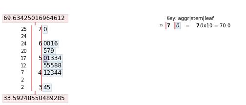
Unlike R where we can simply call the stem() function to create a stem-and-leaf plot, in Python we must first install and import the stemgraphic library.
# pip install stemgraphic
We can limit the output of how many rows get printed in the resulting output by parsing in the .loc() function. So, if we want to print only the first 25 rows, we will access our dataframe, norm_vals['Number'] followed by .loc[0:25].
import stemgraphic

# create stem-and-leaf plot
fig, ax = stemgraphic.stem_graphic(norm_vals['Number'].iloc[0:25])
Matplotlib Library
We must first import the matplotlib library, a most frequently used graphical library for making basic plots in Python. Let us import this library and plot the histogram.
import matplotlib.pyplot as plt
Histograms
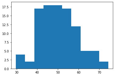
We can proceed to plot a histogram of these norm_vals in order to inspect their distribution from a purely graphical standpoint.
Unlike R, Python does not use a built-in hist() function to accomplish this task. To make the plot, we will parse in our dataframe follows by .hist(grid = False) where grid = False explicitly avoids plotting on a grid. Moreover, plt.show() expressly tells matplotlib to avoid extraneous output above the plot.
# plot a basic histogram
norm_vals['Number'].hist(grid = False)
plt.show()
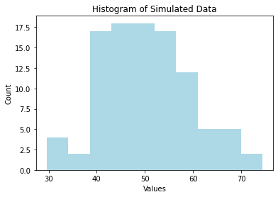
Our title, x-axis, and y-axis labels are given to us by default. However, let us say that we want to change all of them to our desired specifications. To this end, we can parse in and control the following parameters:
norm_vals['Number'].hist(grid=False,
               color = "lightblue") # change color
plt.title ('Histogram of Simulated Data') # title
plt.xlabel('Values')                      # x-axis
plt.ylabel('Count')                       # y-axis
plt.show()
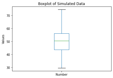
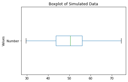
Boxplots
Similarly, we can make a boxplot using the df.boxplot() function call. However, the norm_vals dataframe has two columns. Let us only examine the randomly distributed 100 rows that we have contained in the Number column.
One way to do this is to create a new dataframe to only access the Number column:
norm_number = pd.DataFrame(norm_vals['Number'])
norm_number.boxplot(grid = False)

# plot title
plt.title ('Boxplot of Simulated Data')
# x-axis label
plt.xlabel('')
# y-axis label
plt.ylabel('Values')

plt.show()
Now, let us pivot the boxplot by parsing in the vert=False parameter:
norm_number.boxplot(grid = False, vert = False) # re-orient
plt.title ('Boxplot of Simulated Data') # title
plt.ylabel('Values')                    # y-axis
plt.show()
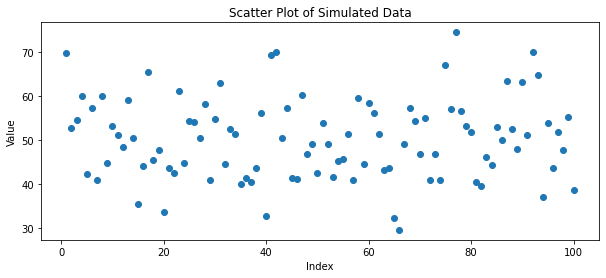
Scatter Plots
To make a simple scatter plot, we will call the plot.scatter() function on the dataframe as follows:
x = norm_vals['Index'] # independent variable
y = norm_vals['Number'] # dependent variable

fig,ax = plt.subplots(figsize = (10,4))
plt.scatter(x, y) # scatter plot call
plt.title('Scatter Plot of Simulated Data')

# we can also separate lines by semicolon
plt.xlabel('Index'); plt.ylabel('Value'); plt.show()
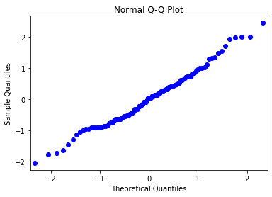
Quantile-Quantile Plot
Let us create a vector from simulated data for the next example and generate a normal quantile plot.
# pip install statsmodels
import statsmodels.api as sm

np.random.seed(222)
quant_ex = np.random.normal(0, 1, 100)

sm.qqplot(quant_ex)
plt.title('Normal Q-Q Plot')
plt.show()
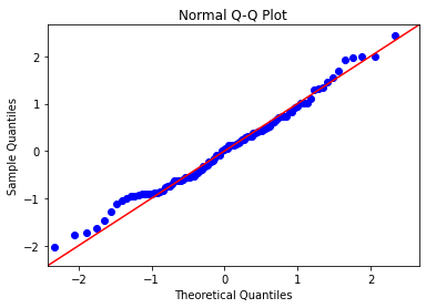
Let us now add a theoretical Q-Q line at a 45 degree angle.
import statsmodels.api as sm

np.random.seed(222)
quant_ex = np.random.normal(0, 1, 100)

sm.qqplot(quant_ex,
          line='45') # theoretical Q-Q line
plt.title('Normal Q-Q Plot')
plt.show()
Skewness and Box-Cox Transformation
From statistics, let us recall that if the mean is greater than the median, the distribution will be positively skewed. Conversely, if the median is greater than the mean, or the mean is less than the median, the distribution will be negatively skewed.
mean_norm_vals = norm_vals['Number'].mean()
median_norm_vals = norm_vals['Number'].median()

print('Mean of norm_vals:', mean_norm_vals)
print('Median of norm_vals:', median_norm_vals)

print('Difference =', mean_norm_vals - median_norm_vals)
Since both the mean and the median values are fairly close together, the data appears to be normally distributed, so we will simulate another example involving skewness.
Whereas in R, we use the all-encompassing caret machine learning library to handle multiple tasks, often we find ourselves loading more libraries in Python like the scipy library to handle Box-Cox transformations.
# pip install scipy
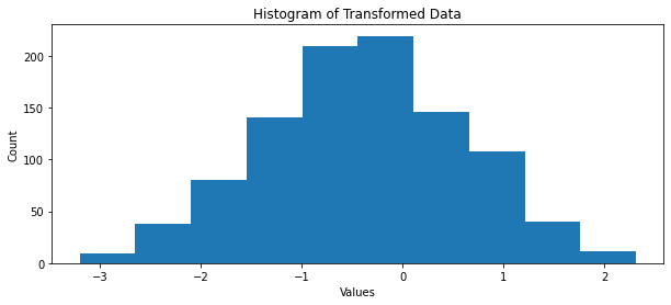
from scipy import stats
original_data = np.random.exponential(size = 1000)

# transform training data & save lambda value
fitted_data, fitted_lambda = stats.boxcox(original_data)
original_data1 = pd.DataFrame(original_data)
fitted_data1 = pd.DataFrame(fitted_data)
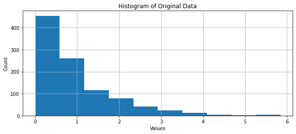
# original hist(0)
original_data1.hist(figsize=(10,4))
plt.title ('Histogram of Original Data')
plt.xlabel('Values'); plt.ylabel('Count')

# transformed hist()
fitted_data1.hist(grid = False,
                  figsize=(10,4))
plt.title ('Histogram of Transformed Data')
plt.xlabel('Values'); plt.ylabel('Count')
plt.show()
Basic Modeling
Simple Linear Regression
Let us set up an example dataset for the following modeling endeavors.
We will be accessing Python's most commonly used machine learning library, scikit-learn to build the ensuing algorithms, though there are others like pycaret and SciPy, to name a few.
So, let us go ahead and import sklearn for linear regression into our environment.
# pip install sklearn
Notice a more refined importing syntax, atypical of the standard import library name. We are telling Python to import the Linear Regression module from the scikit-learn library as follows:
from sklearn.linear_model import LinearRegression
lin_mod = pd.DataFrame({
                # X1
                'Hydrogen':[.18,.20,.21,.21,.21,.22,.23,
                            .23,.24,.24,.25,.28,.30,.37,.31,
                            .90,.81,.41,.74,.42,.37,.49,.07,
                            .94,.47,.35,.83,.61,.30,.61,.54],
                # X2
                'Oxygen':[.55,.77,.40,.45,.62,.78,.24,.47,
                          .15,.70,.99,.62,.55,.88,.49,.36,
                          .55,.42,.39,.74,.50,.17,.18,.94,
                          .97,.29,.85,.17,.33,.29,.85],
                # X3
                'Nitrogen':[.35,.48,.31,.75,.32,.56,.06,.46,
                            .79,.88,.66,.04,.44,.61,.15,.48,
                            .23,.90,.26,.41,.76,.30,.56,.73,
                            .10,.01,.05,.34,.27,.42,.83],
                # y
                'Gas Porosity':[.46,.70,.41,.45,.55,
                                .44,.24,.47,.22,.80,.88,.70,
                                .72,.75,.16,.15,.08,.47,.59,
                                .21,.37,.96,.06,.17,.10,.92,
                                .80,.06,.52,.01,.37]})
lin_mod
x1 = lin_mod['Hydrogen']; x2 = lin_mod['Oxygen']
x3 = lin_mod['Nitrogen']; y = lin_mod['Gas Porosity']
Prior to modeling, it is best practice to examine correlation visa vie visual scatterplot analysis as follows:
fig,ax = plt.subplots(figsize = (10,4)) # resize plot
plt.scatter(x1, y)
plt.title('Gas Porosity vs. Hydrogen')
plt.xlabel('Hydrogen Content'); plt.ylabel('Gas Porosity')
plt.show()
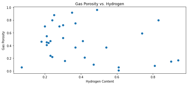
Now let us calculate our correlation coefficient for the first variable relationship.
corr1 = np.corrcoef(x1, y)
r1 = corr1[0,1]
r1
By the correlation coefficient r you will see that there exists a relatively moderate (positive) relationship. Let us now build a simple linear model from this dataframe.
# notice the additional brackets
# we do this to specify columns
# within our dataframe of interest
X1 = lin_mod[['Hydrogen']]
y = lin_mod[['Gas Porosity']]

# set-up the linear regression
lm_model1 = LinearRegression().fit(X1, y)
Next, we will rely on the stats model package to obtain a summary output table. Here, it is important to note that unlike in R, the statsmodels package in Python does not add a constant to the summary output, so for reproducible results, we will add it by the sm.add_constant() function.
from statsmodels.api import OLS
X1 = sm.add_constant(X1)
X1_results = OLS(y,X1).fit()
X1_results.summary()
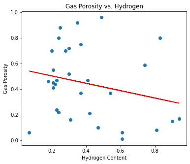
Notice how the p-value for hydrogen content is 0.196, which lacks statistical significance when compared to the alpha value of 0.05 (at the 95% confidence level). Moreover, the R-Squared value of 0.057 suggests that roughly 6% of the variance for gas propensity is explained by hydrogen content.
We can make the same scatter plot, but this time with a best fit line.
fig, ax = plt.subplots(figsize=(6,5))
plt.scatter(x1, y)
plt.title('Gas Porosity vs. Hydrogen')
plt.xlabel('Hydrogen Content')
plt.ylabel('Gas Porosity')

# create best-fit line based on slope-intercept form
m, b = np.polyfit(x1, y, 1)
plt.plot(x1, m*x1 + b,
         color = 'red')

plt.show()
Multiple Linear Regression
To account for all independent (x) variables in the model, let us set up the model in a dataframe:
X = lin_mod[['Hydrogen', 'Oxygen', 'Nitrogen']]
y = lin_mod[['Gas Porosity']]
Let us plot the remaining variable relationships.
fig, ax = plt.subplots(figsize=(6,5))
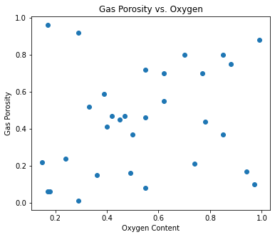
plt.scatter(x2,y)
plt.title('Gas Porosity vs. Oxygen')
plt.xlabel('Oxygen Content')
plt.ylabel('Gas Porosity')
plt.show()
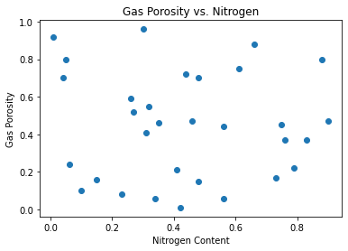
x3_plot =plt.scatter(x3,y) # create scatter plot
plt.title('Gas Porosity vs. Nitrogen') # title
plt.xlabel('Nitrogen Content')       # x-axis label
plt.ylabel('Gas Porosity')           # y-axis label
x3_plot
plt.show()
X = sm.add_constant(X)
lin_model_results = OLS(y,X).fit()
lin_model_results.summary()
Logistic Regression
Whereas in linear regression, it is necessary to have a quantitative and continuous target variable, logistic regression is part of the generalized linear model series that has a categorical (often binary) target (outcome) variable. For example, let us say we want to predict grades for mathematics courses taught at a university. So, we have the following example dataset:
math_df = pd.DataFrame(
    {'Calculus1':[56,80,10,8,20,90,38,42,57,58,90,2,
                  34,84,19,74,13,67,84,31,82,67,99,
                  76,96,59,37,24,3,57,62],
     'Calculus2':[83,98,50,16,70,31,90,48,67,78,55,
                  75,20,80,74,86,12,100,63,36,91,
                  19,69,58,85,77,5,31,57,72,89],
     'linear_alg':[87,90,85,57,30,78,75,69,83,85,90,
                   85,99,97, 38,95,10,99,62,47,17,
                   31,77,92,13,44,3,83,21,38,70],
     'pass_fail':['P','F','P','F','P','P','P','P',
                  'F','P','P','P','P','P','P','F',
                  'P','P','P','F','F','F','P','P',
                  'P','P','P','P','P','P','P']})
math_df
At this juncture, we cannot build a model with categorical values until and unless they are binarized using a dictionary mapping. A passing score will be designated by a 1, and failing score with a 0, respectively.
# binarize pass fail to 1 = pass, 0=fail
# into new column
math_df['math_outcome'] = math_df['pass_fail'].map({'P':1,'F':0})
math_df
Let us import the Linear Regression module from the scikit-learn library as follows:
from sklearn.linear_model import LogisticRegression
Instead of OLS.fit() like we did for linear regression, we will be using the sm.Logit() function call to pass in our y and x, respectively.
# we can also drop the columns that we
# will not be using
logit_X = math_df.drop(columns=['pass_fail',
                                'math_outcome'])
logit_X = sm.add_constant(logit_X)
logit_y = math_df['math_outcome']

# notice the sm.Logit() function call
log_results = sm.Logit(logit_y,logit_X).fit()
log_results.summary()
Decision Trees
Let us import the Decision Tree Classifier from scikit-learn.
from sklearn import tree
from sklearn.tree import DecisionTreeClassifier
We will be using the mtcars dataset from R, and will have to import from statsmodels into Python first.
mtcars = sm.datasets.get_rdataset("mtcars", "datasets", cache=True).data
mtcars = pd.DataFrame(mtcars)
mtcars
print(mtcars.dtypes, '\n')
print('Number of Rows:',mtcars.shape[0])
print('Number of Columns:',mtcars.shape[1])
# convert from float to int
# otherwise DT won't run properly
mtcars = mtcars.astype(int)
print(mtcars.dtypes, '\n')
print('Number of Rows:',mtcars.shape[0])
print('Number of Columns:',mtcars.shape[1])
Similar to what we did for the logistic regression example, let us now create our x and y variables from this mtcars dataset.
mtcars_X = mtcars.drop(columns=['mpg'])
mtcars_y = mtcars[['mpg']]
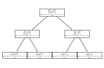
Without importing any special graphical libraries, the decision tree output plot will look condensed, small, and virtually unreadable. We can comment out the figure size dimensions, but that still will not produce anything sophisticated in nature.
# fig,ax = plt.subplots(figsize = (30,30))
tree_model = DecisionTreeClassifier(max_depth=2)
tree_model = tree_model.fit(mtcars_X, mtcars_y)
tree_plot = tree.plot_tree(tree_model)
Another way to label our x and y variables is to assign the x variables to a list and use the .remove() function to remove our target variable from that list.
X_var = list(mtcars.columns)
target = 'mpg'
X_var.remove(target)
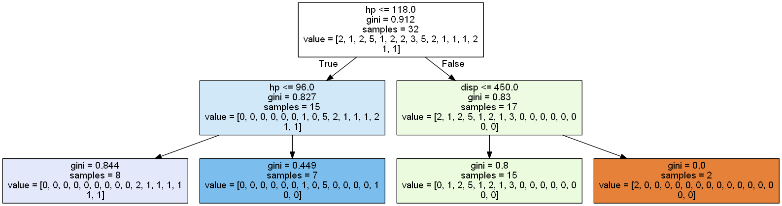
For a more sophisticated graphical output, we can tap into scikit-learn's export_graphviz package in conjunction with another library called pydotplus which we will need to install separately.
# pip install pydotplus
from sklearn.tree import export_graphviz
import pydotplus
from IPython.display import Image
dot_data = export_graphviz(tree_model,
                           feature_names = X_var,
                           filled = True,
                           out_file = None)
graph = pydotplus.graph_from_dot_data(dot_data)
Image(graph.create_png())
Basic Modeling and Cross-Validation in Python
from sklearn.model_selection import train_test_split
X_train, X_test, y_train, \
y_test = train_test_split(mtcars_X, mtcars_y,
                          test_size = 0.25,
                          random_state = 222)
# get the shape of train and test sets
train_shape = X_train.shape[0]
test_shape = X_test.shape[0]

# calculate the proportions of each, respectively
train_percent = train_shape/(train_shape + test_shape)
test_percent = test_shape/(train_shape + test_shape)

print('Train Size:', train_percent)
print('Test Size:', test_percent)
Let us bring in a generalized linear model for this illustration.
mtcars_X = mtcars.drop(columns=['mpg'])
mtcars_y = mtcars[['mpg']]

# notice the sm.Logit() function call
mtcars_model = sm.add_constant(X_train)

# back to the linear model since target
# variable is quantitative and continuous
mtcars_model_results = OLS(y_train, X_train).fit()
mtcars_model_results.summary()
Before we can cross-validate, let us run our predictions of miles per gallon (mpg) on our holdout (test-set).
mtcars_mod = LinearRegression()
mtcars_mod.fit(X_train, y_train)
y_pred = mtcars_mod.predict(X_test)
y_pred
While our predictions remain nested in an array, we will bring in a baseline measure from the scikit-learn library as follows:
from sklearn.metrics import mean_absolute_error
mean_absolute_error(y_test, y_pred)
from sklearn.model_selection import cross_val_score
from sklearn.model_selection import KFold
from numpy import mean
from numpy import absolute
# define cross-validation method to use
cv = KFold(n_splits=5, random_state=222, shuffle=True)

# use k-fold CV to evaluate model
scores = cross_val_score(mtcars_mod, X_train, y_train,
                         scoring='neg_mean_absolute_error',
                         cv=cv, n_jobs=-1)

# view mean absolute error
ma_scores = mean(absolute(scores))
ma_scores
K-Means Clustering
A cluster is a collection of observations. We want to group these observations based on the most similar attributes. We use distance measures to measure similarity between clusters. This is one of the most widely-used unsupervised learning techniques that groups "similar data points together and discover underlying patterns. To achieve this objective, K-means looks for a fixed number (k) of clusters in a dataset" (Garbade, 2018).
The k in k-means is the fixed number of centroids (center of cluster) for which the algorithm will take the mean for based on the number of clusters (collection of data points).
# import the necessary library
from sklearn.cluster import KMeans
Let us split the mtcars dataset into 3 clusters.
kmeans = KMeans(n_clusters=3).fit(mtcars)
centroids = kmeans.cluster_centers_
print(centroids)
kmeans1 = KMeans(n_clusters=3,
                 random_state=222).fit(mtcars)
centroids1 = pd.DataFrame(kmeans1.cluster_centers_,
columns = mtcars.columns)
pd.set_option('precision', 3)
centroids1
withinClusterSS = [0] * 3
clusterCount = [0] * 3
for cluster, distance in zip(kmeans1.labels_,
                             kmeans1.transform(mtcars)):
    withinClusterSS[cluster] += distance[cluster]**2
    clusterCount[cluster] += 1
for cluster, withClustSS in enumerate(withinClusterSS):
    print('Cluster {} ({} members): {:5.2f} within cluster'.format(cluster,
clusterCount[cluster], withinClusterSS[cluster]))
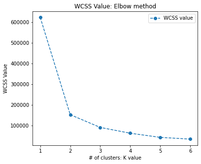
But what is the appropriate number of clusters that we should generate? Can we do better with more clusters?
# let's create segments using K-means clustering
# using elbow method to find no of clusters
wcss=[]
for i in range(1,7):
    kmeans= KMeans(n_clusters = i,
                   init = 'k-means++',
                   random_state = 222)
    kmeans.fit(mtcars_X)
    wcss.append(kmeans.inertia_)
print(wcss)

fig, ax = plt.subplots(figsize=(6,5))
plt.plot(range(1,7),
         wcss, linestyle='--',
         marker='o',
         label='WCSS value')
plt.title('WCSS Value: Elbow method')
plt.xlabel('# of clusters: K value')
plt.ylabel('WCSS Value')
plt.legend()
plt.show()
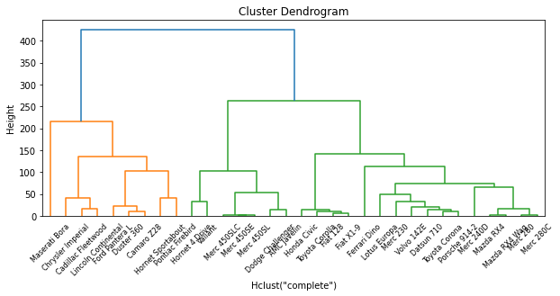
Hierarchical Clustering
This is another form of unsupervised learning type of cluster analysis, which takes on a more visual method, working particularly well with smaller samples (i.e., n < 500), such as this mtcars dataset. We start out with as many clusters as observations, and we go through a procedure of combining observations into clusters, culminating with combining clusters together as a reduction method for the total number of clusters that are present.
Moreover, the premise for combining clusters together is a direct result of:
complete linkage - largest Euclidean distance between clusters.
single linkage - conversely, we look at the observations which are closest together (proximity).
centroid linkage - we can the distance between the centroid of each cluster.
group average (mean) linkage - taking the mean between the pairwise distances of the observations.
Complete linkage is the most traditional approach, so we parse in the method='complete' hyperparameter.
The tree structure that examines this hierarchical structure is called a dendogram.
import scipy.cluster.hierarchy as shc
plt.figure(figsize=(10, 4))
dend = shc.dendrogram(shc.linkage(mtcars, method='complete'),
                                  labels=list(mtcars.index))
plt.title("Cluster Dendrogram"); plt.xlabel('Hclust("complete")')
plt.ylabel('Height');plt.show()
Sources
finnstats. (2021, October 31). What Does Cross Validation Mean? R-bloggers.
https://www.r-bloggers.com/2021/10/cross-validation-in-r-with-example/
Garbade, Michael. (2018, September 12). Understanding K-means Clustering in
Machine Learning. Towards Data Science.
https://towardsdatascience.com/understanding-k-means-clustering-in-machine
-learning-6a6e67336aa1
GeeksforGeeks. (2020, April 22). Scope of Variable in R. GeeksforGeeks.
https://www.geeksforgeeks.org/scope-of-variable-in-r/
Shmueli, G., Bruce, P. C., Gedeck, P., & Patel, N. R. (2020). Data mining for
business analytics: Concepts, techniques and applications in Python. Wiley.