NIOSH - Data Science for Everyone Workshop - Accidents Data Case Study (Python)
Created by Leonid Shpaner for use in NIOSH - Data Science for Everyone Workshop. The dataset originates for Data Mining from Business Analytics (Shmueli et., 2018). The functions and syntax are presented in the most basic format to facilitate ease of use.
The Accidents dataset is presented as a flat .csv file which is comprised of 42,183 recorded automobile
accidents from 2001 in the United States. The following three outcomes are observed: “NO INJURY,
INJURY, or FATALITY.” Each accident is supplemented with additional information (i.e., day of the week,
condition of weather, and road type). This may be of interest to an organization looking to develop “a
system for quickly classifying the severity of an accident based on initial reports and associated data in the
system (some of which rely on GPS-assisted reporting)” (Shmueli et al., 2018, p. 202).
Loading, Pre-Processing, and Exploring Data
Let's make sure the dataset is in the same path as our Python script. If you save the
data somewhere else, you need to pass in the full path to where you saved the dataset, e.g. dataset = pd.read_csv('C:/Downloads/dataset.csv').
Let's install the necessary libraries first, uncommenting (removing the # symbol) in front of the commands in the cell blocks, and then running them, respectively.
# pip install pandas; pip install statsmodels; pip install sklearn
# pip install pydotplus; pip install prettytable
Now, let's load these necessary libraries as follows:
import pandas as pd
import numpy as np
import matplotlib.pyplot as plt
import seaborn as sns
from prettytable import PrettyTable
import statsmodels.api as sm
from sklearn.model_selection import train_test_split
from sklearn import metrics
from sklearn.metrics import roc_curve, auc, mean_squared_error,\
precision_score, recall_score, f1_score, accuracy_score,\
confusion_matrix, plot_confusion_matrix, classification_report
from sklearn.linear_model import LogisticRegression
from sklearn.tree import DecisionTreeClassifier, export_graphviz
from sklearn.ensemble import RandomForestClassifier
import warnings
warnings.filterwarnings('ignore')
Now, we proceed to read in the flat .csv file, and examine the first 4 rows of data.
url = 'https://raw.githubusercontent.com/lshpaner/data_science_\
for_everyone/main/Case%20Study/accidentsFull.csv'
accidents = pd.read_csv(url)
Now let's inspect the dataset.
accidents.head(4)
Data Dictionary
Prior to delving deeper, let us first identify (describe) what each respective variable name really means. To this end, we have the following data dictionary:
- HOUR_I_R - rush hour classification: 1 = rush hour, 0 = not rush hour (rush hour = 6-9 am, or 4-7 pm)
- ALCHL_I - alcohol involvement: Alcohol involved = 1, alcohol not involved = 2
- ALIGN_I - road alignment: 1 = straight, 2 = curve
- STRATUM_R - National Automotive Sampling System stratum: 1 = NASS Crashes involving at least one passenger vehicle (i.e., a passenger car, sport utility Vehicle, pickup truck or van) towed due to damage from the crash scene and no medium or heavy trucks are involved. 0 = not
- WRK_ZONE - work zone: 1= yes, 0 = no
- WKDY_I_R - weekday or weekend: 1 = weekday, 0 = weekend
- INT_HWY - interstate highway: 1 =yes, 0 = no
- LGTCON_I_R - light conditions - 1=day, 2=dark (including dawn/dusk), 3 = dark, but lighted, 4 = dawn or dusk
- MANCOL_I - type of collision: 0 = no collision, 1 = head-on, 2 = other form of collision
- PED_ACC_R - collision involvement type: 1=pedestrian/cyclist involved, 0=not
- RELJCT_I_R - whether the collision occurred at intersection: 1=accident at intersection/interchange, 0=not at intersection
- REL_RWY_R - related to roadway or not: 1 = accident on roadway, 0 = not on roadway
- PROFIL_I_R - road profile: 1 = level, 0 = other
- SPD_LIM - speed limit, miles per hour: numeric
- SUR_CON - surface conditions (1 = dry, 2 = wet, 3 = snow/slush, 4 = ice, 5 = sand/dirt/oil, 8 = other, 9 = unknown)
- TRAF_CON_R - traffic control device: 0 = none, 1 = signal, 2 = other (sign, officer, . . . )
- TRAF_WAY - traffic type: 1 = two-way traffic, 2 = divided hwy, 3 = one-way road
- VEH_INVL - vehicle involvement: number of vehicles involved (numeric)
- WEATHER_R - weather conditions: 1=no adverse conditions, 2=rain, snow or other adverse condition
- INJURY_CRASH - injury crash: 1 = yes, 0 = no
- NO_INJ_I - number of injuries: numeric
- PRPTYDMG_CRASH - property damage: 1 = property damage, 2 = no property damage
- FATALITIES - fatalities: 1 = yes, 0 = no
- MAX_SEV_IR - maximum severity: 0 = no injury, 1 = non-fatal injury, 2 = fatal injury
Initial Pre-Processing Steps
Speed limit (SPD_LIM) has valuable numerical information, so let us go ahead and create buckets for this data.
unique_speed = accidents['SPD_LIM'].unique()
unique_speed.sort()
unique_speed = pd.DataFrame(unique_speed)
unique_speed.T
labels = [ "{0} - {1}".format(i, i + 5) for i in range(0, 100, 10) ]
accidents['MPH Range'] = pd.cut(accidents.SPD_LIM, range(0, 105, 10),
                                right=False,
                                labels=labels)
# inspect the new dataframe with this info
accidents[['SPD_LIM', 'MPH Range']]
accidents['MPH Range'] = accidents['SPD_LIM'].map({5:'5-10', 10:'5-10',
                                                   15: '15-20', 20:'15-20',
                                                   25: '25-30', 30: '25-30',
                                                   35: '35-40', 40: '35-40',
                                                   45: '45-50', 50: '45-50',
                                                   55: '55-60', 60: '55-60',
                                                   65: '65-70', 70: '65-70',
                                                   75: '75'})
accidents['MPH Range']
Next, we create a dummy variable called INJURY to determine if the accident resulted in an injury based on maximum severity. So, if the severity of the injury is greater than zero, we specify yes. Otherwise, we specify no.
accidents['INJURY'] = np.where(accidents['MAX_SEV_IR'] > 0, 'yes', 'no')
accidents.head()
Exploratory Data Analysis
Let us first examine the structure of this dataset so we can gather the details about the size, shape, and values of the dataframe holistically, and each column, respectively.
print('Number of Rows:', accidents.shape[0])
print('Number of Columns:', accidents.shape[1], '\n')

data_types = accidents.dtypes
data_types = pd.DataFrame(data_types)
data_types = data_types.assign(Null_Values =
                               accidents.isnull().sum())
data_types.reset_index(inplace = True)
data_types.rename(columns={0:'Data Type',
                          'index': 'Column/Variable',
                          'Null_Values': "# of Nulls"})
How many accidents resulted in injuries? We create a stylistic pandoc table from the PrettyTable() library to
inspect these results.
injury_yes = accidents['INJURY'].value_counts()['yes']
injury_no = accidents['INJURY'].value_counts()['no']
injury_total = injury_yes + injury_no

table1 = PrettyTable() # build a table
table1.field_names = ['Yes: Injured', 'No: Uninjured',
                      'Total Injured']
table1.add_row([injury_yes, injury_no, injury_total])
print(table1)
What percentage of accidents resulted in injuries?
perc_inj = injury_yes/(injury_yes + injury_no)
print(round(perc_inj, 2)*100, '% of accidents'
                       ' resulted in injuries')
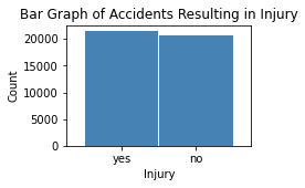
A little more than half of the accidents resulted in injuries; thus, we should intrinsically focus our predictions in favor of injuries. However, predictive analytics requires more than merely a cursory glance at first tier probability results. Therefore, we cannot make any assumptions at face value. We will proceed to model this behavior later, but for now let us continue exploring the data.
# accidents injury bar graph
injury_count = accidents['INJURY'].value_counts()
fig = plt.figure(figsize=(3,2))
injury_count.plot.bar(x ='lab', y='val', rot=0, width=0.99,
                         color="steelblue")
plt.title ('Bar Graph of Accidents Resulting in Injury')
plt.xlabel('Injury')
plt.ylabel('Count')
plt.show()
accidents.dtypes
print("\033[1m"+'Injury Outcomes by Miles per Hour'+"\033[1m")

def INJURY_by_MPH():

    INJURY_yes = accidents.loc[accidents.INJURY == 'yes'].groupby(
                               ['MPH Range'])[['INJURY']].count()

    INJURY_yes.rename(columns = {'INJURY':'Yes'}, inplace=True)

    INJURY_no = accidents.loc[accidents.INJURY == 'no'].groupby(
                               ['MPH Range'])[['INJURY']].count()

    INJURY_no.rename(columns = {'INJURY':'No'}, inplace=True)

    INJURY_comb = pd.concat([INJURY_yes, INJURY_no], axis = 1)

    # sum row totals
    INJURY_comb['Total'] = INJURY_comb.sum(axis=1)
    INJURY_comb.loc['Total'] = INJURY_comb.sum(numeric_only = True,
                                               axis=0)
    # get % total of each row
    INJURY_comb['% Injured'] = round((INJURY_comb['Yes'] /
                                      (INJURY_comb['Yes']
                                     + INJURY_comb['No']))* 100, 2)

    return INJURY_comb.style.format("{:,.0f}")

INJURY_by_MPH()
mph_inj = INJURY_by_MPH().data # retrieve dataframe
mph_inj
mph_plt = mph_inj['Total'][0:8].sort_values(ascending=False)
mph_plt.plot(kind='bar', width=0.90)
plt.title('Accidents by Speed Limit')
plt.xlabel('Speed Limit (in MPH)')
plt.ylabel('# of Accidents')
plt.show()
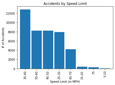
Note. The 35-40 mph speed limit shows the highest prevalence of accidents.
fig = plt.figure(figsize=(8,8))
ax1 = fig.add_subplot(211)
ax2 = fig.add_subplot(212)
fig.tight_layout(pad=6)

mph_plt2 = mph_inj[['Yes', 'No']][0:8].sort_values(by=['Yes'],
                                                   ascending=False)
mph_plt2.plot(kind='bar', stacked=True,
              ax=ax1, color = ['#F8766D', '#00BFC4'], width = 0.90)
ax1.set_title('Speed Limit by Injury Outcome: (Injured or Not)')
ax1.set_xlabel('Speed Limit (in Miles per Hour)')
ax1.set_ylabel('Count')

# normalize the plot and plot it
mph_plt_norm = mph_plt2.div(mph_plt2.sum(1), axis = 0)
mph_plt_norm.plot(kind='bar', stacked=True,
                  ax=ax2,color = ['#F8766D', '#00BFC4'], width = 0.90)
ax2.set_title('Speed Limit by Injury Outcome: (Injured or Not): Normalized')
ax2.set_xlabel('Speed Limit (in Miles per Hour)')
ax2.set_ylabel('Frequency')

plt.show()
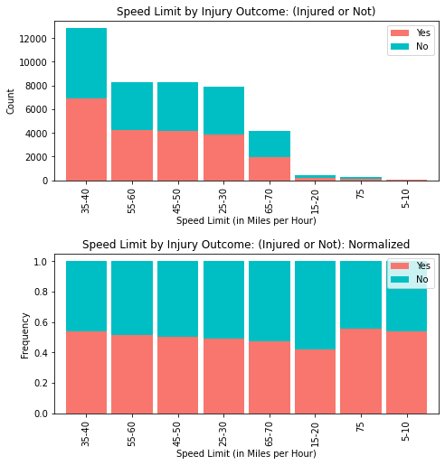
From the speed limit group bar graph overlayed with “injured” and “non-injured” accident results, it is evident that the speed limit of 35-40 mph has a greater incidence of injuries (more than any other speed limit group).
While the strength of this graph is in its depiction of the overall distribution (providing us with injuries vs. non-injuries in each speed related accident), it does little to provide a comparison of the frequency (incidence rate) of injuries among the speed limit groups.
Normalizing the speed limit groups by our target (INJURY) assuages this analysis in such capacity. From here, it is easier to see that speed limits of 5-10 miles per hour, and 35-40 miles per hour, respectively had roughly 50% injury rates, whereas (notably), 75 miles per hour exhibited the highest injury rate of all.
Note. There are precisely 12,845 accidents that occurred between the 35-40 mph speed limit. 6,873 (or 53.51%) of them resulted in injuries. Now, let us plot the histogram distributions from each respective variable of the dataset. Figure 3 below visually illustrates these distributions.
Histogram Distributions
# checking for degenerate distributions
accidents.hist(grid=False, figsize=(16,15))

plt.show()
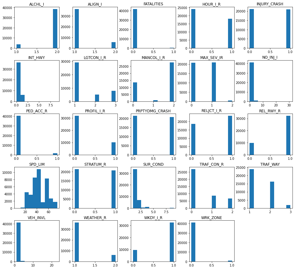
23 out of the original 24 variables are categorical, and from the histograms presented herein it is possible to uncover degenerate distributions with relative ease, as one category represents higher values over another. However, we look to the speed limit as the sole quantitative predictor which yields a positively skewed distribution. The following summary statistics corroborate this claim since the mean of 44 is greater than the median of 40.
summ_stats = pd.DataFrame(accidents['SPD_LIM'].describe()).T
summ_stats
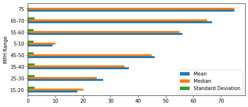
print("\033[1m"+'Accidents by Speed Limit Summary'+"\033[1m")
def accident_stats_by_mph():
    pd.options.display.float_format = '{:,.2f}'.format
    new2 = accidents.groupby('MPH Range')['SPD_LIM']\
    .agg(["mean", "median", "std", "min", "max"])
    new2.loc['Total'] = new2.sum(numeric_only=True, axis=0)
    column_rename = {'mean': 'Mean', 'median': 'Median',
                     'std': 'Standard Deviation',\
                     'min':'Minimum','max': 'Maximum'}
    dfsummary = new2.rename(columns = column_rename)
    return dfsummary
acc_stats_mph = accident_stats_by_mph()
accident_stats_by_mph()
acc_stats_mph.iloc[:, 0:3][0:8].plot.barh(figsize=(8,3.5))
plt.show()
Selected Boxplot Distribution - Speed Limit
# selected boxplot distributions
print("\033[1m"+'Boxplot Distribution'+"\033[1m")

# Boxplot of age as one way of showing distribution
fig = plt.figure(figsize = (10,1.5))
plt.title ('Boxplot: Speed Limit')
plt.xlabel('Speed Limit')
plt.ylabel('Value')
sns.boxplot(data=accidents['SPD_LIM'],
            palette="coolwarm", orient='h',
            linewidth=2.5)
plt.show()

IQR = summ_stats['75%'][0] - summ_stats['25%'][0]

print('The first quartile is %s. '%summ_stats['25%'][0])
print('The third quartile is %s. '%summ_stats['75%'][0])
print('The IQR is %s.'%round(IQR,2))
print('The mean is %s. '%round(summ_stats['mean'][0],2))
print('The standard deviation is %s. '%round(summ_stats['std'][0],2))
print('The median is %s. '%round(summ_stats['50%'][0],2))
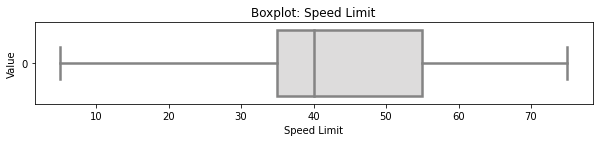
\ Whereas no outliers are present in the speed limit variable, there exists some skewness where the mean (43.55) is slightly greater than the median (40.00). Whereas typically a Box-Cox transformation could mitigate against skewness by transforming the variable(s) of interest, we will not be making such transformation to avoid misrepresenting the speed limit variable.
Correlation Matrix
# correlation matrix title
print("\033[1m"+'Accidents Data: Correlation Matrix'+"\033[1m")

# assign correlation function to new variable
corr = accidents.corr()
matrix = np.triu(corr) # for triangular matrix
plt.figure(figsize=(20,20))
# parse corr variable intro triangular matrix
sns.heatmap(accidents.corr(method='pearson'),
            annot=True, linewidths=.5,
            cmap="coolwarm", mask=matrix,
            square = True,
            cbar_kws={'label': 'Correlation Index'})
plt.show()
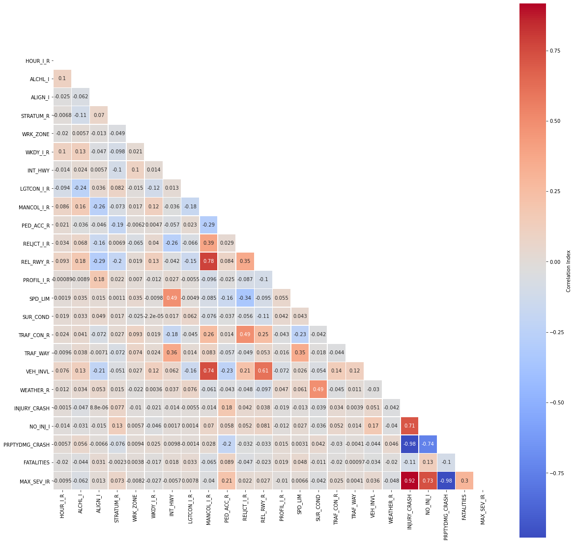
Multicollinearity
Let us narrow our focus by removing highly correlated predictors and passing the rest into a new dataframe.
cor_matrix = accidents.corr().abs()
upper_tri = cor_matrix.where(np.triu(np.ones(cor_matrix.shape),
                                     k=1).astype(np.bool))

to_drop = [column for column in upper_tri.columns if
           any(upper_tri[column] > 0.75)]
print('These are the columns we should drop: %s'%to_drop)
accidents_1 = accidents.drop(columns=['MPH Range','NO_INJ_I','INJURY',
                                      'INJURY_CRASH', 'MANCOL_I_R',
                                      'FATALITIES', 'INT_HWY', 'TRAF_WAY'])
accidents_1 = accidents_1.drop(to_drop, axis=1)
print(accidents_1.dtypes, '\n')
print('Number of Rows:', accidents_1.shape[0])
print('Number of Columns:', accidents_1.shape[1])
Additional Pre-Processing
MPH_Range was created strictly for exploratory data analysis purposes. The INJURY column was based off the maximum injury severity column MAX_SEV_IR, so, we will binarize the INJURY column into a new Injured column in lieu of the prior two.
accidents['Injured'] = accidents['INJURY'].map({'yes':1, 'no':0})
Furthermore, we must remove the REL_RWY_R, PRPTYDMG_CRASH, and MAX_SEV_IR columns from the dataframe resulting from the inherent between-predictor and predictor-target relationships, respectively. However, there are still a few predictors that warrant subsequent omission. Number of injuries (NO_INJ_I) and fatalities (FATALATIES) are inherently and intrinsically related to the outcome by virtue of their meaning. Therefore, in order to avoid overfitting the model, we remove them.
accidents_1 = accidents.drop(columns=['MPH Range','NO_INJ_I','INJURY',
                                      'INJURY_CRASH', 'MANCOL_I_R',
                                      'FATALITIES'])
accidents_1 = accidents_1.drop(to_drop, axis=1)
print(accidents_1.dtypes, '\n')
print('Number of Rows:', accidents_1.shape[0])
print('Number of Columns:', accidents_1.shape[1])
Checking for Statistical Significance Via Baseline Model
The logistic regression model is introduced as a baseline because establishing impact of coefficients on each independent feature can be carried with relative ease. Moreover, it is possible to gauge statistical significance from the reported p-values of the summary output table below.
Generalized Linear Model - Logistic Regression Baseline
Logistic Regression - Parametric Form
Logistic Regression - Descriptive Form
X = accidents_1.drop(columns=['Injured'])
X = sm.add_constant(X)
y = pd.DataFrame(accidents_1[['Injured']])
log_results = sm.Logit(y,X, random_state=222).fit()
log_results.summary()
From the summary output table, we observe that WRK_ZONE, INT_HWY, LGTCON_I_R, and TRAF_WAY have p-values of 0.168, 0.173, and 0.757, respectively, thereby ruling out statistical significance where α = 0.05. We will thus remove them from the refined dataset.
accidents1 = accidents_1.drop(columns=['WRK_ZONE','INT_HWY',
                          'LGTCON_I_R', 'TRAF_WAY'])
Train_Test_Split
X = accidents_1.drop(columns=['Injured'])
y = pd.DataFrame(accidents_1['Injured'])

X_train, X_test, y_train, y_test = train_test_split(X, y,
                                   test_size=0.20, random_state=42)

# confirming train_test_split proportions
print('training size:', round(len(X_train)/len(X),2))
print('test size:', round(len(X_test)/len(X),2))
# confirm dimensions (size of newly partioned data)
print('Training:', len(X_train))
print('Test:', len(X_test))
print('Total:',   len(X_train)
                + len(X_test))
Model Building Strategies
Logistic Regression
# Un-Tuned Logistic Regression Model
logit_reg = LogisticRegression(random_state=222)
logit_reg.fit(X_train, y_train)
# Predict on test set
logit_reg_pred1 = logit_reg.predict(X_test)
# accuracy and classification report
print('Untuned Logistic Regression Model')
print('Accuracy Score')
print(accuracy_score(y_test, logit_reg_pred1))
print('Classification Report \n',
classification_report(y_test, logit_reg_pred1))
# Tuned Logistic Regression Model
C = [0.01, 0.1, 0.5, 1, 5, 10, 50]
LRtrainAcc = []
LRtestAcc = []
for param in C:
tuned_lr = LogisticRegression(solver = 'saga',
C = param,
max_iter = 200,
n_jobs = -1,
random_state = 222)
tuned_lr.fit(X_train, y_train)
# Predict on train set
tuned_lr_pred_train = tuned_lr.predict(X_train)
# Predict on test set
tuned_lr1 = tuned_lr.predict(X_test)
LRtrainAcc.append(accuracy_score(y_train, tuned_lr_pred_train))
LRtestAcc.append(accuracy_score(y_test, tuned_lr1))
# accuracy and classification report
print('Tuned Logistic Regression Model')
print('Accuracy Score')
print(accuracy_score(y_test, tuned_lr1))
print('Classification Report \n',
classification_report(y_test, tuned_lr1))
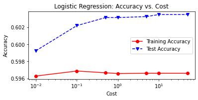
# plot cost by accuracy
fig, ax = plt.subplots(figsize=(6,2.5))
ax.plot(C, LRtrainAcc, 'ro-', C, LRtestAcc,'bv--')
ax.legend(['Training Accuracy','Test Accuracy'])
plt.title('Logistic Regression: Accuracy vs. Cost')
ax.set_xlabel('Cost'); ax.set_xscale('log')
ax.set_ylabel('Accuracy'); plt.show()
Decision Trees
Before we print the classification report for the un-tuned decision tree, let us establish the optimal maximum depth hyperparameter by varying it in a for-loop as follows:
# Vary the decision tree depth in a loop,
# increasing depth from 3 to 14.

accuracy_depth=[]

for depth in range(3,15):

    varied_tree = DecisionTreeClassifier(max_depth = depth,
                                         random_state = 222)
    varied_tree=varied_tree.fit(X_train,y_train)
    tree_test_pred = varied_tree.predict(X_test)
    tree_train_pred = varied_tree.predict(X_train)
    accuracy_depth.append({'depth':depth,
                           'test_accuracy':accuracy_score\
                           (y_test,tree_test_pred),
                           'train_accuracy':accuracy_score\
                           (y_train,tree_train_pred)
                          })

    print('Depth = %2.0f \t Test Accuracy = %2.2f \t \
    Training Accuracy = %2.2f'% (depth,accuracy_score\
                                (y_test, tree_test_pred),
                                 accuracy_score(y_train,
                                 tree_train_pred)))

abd_df = pd.DataFrame(accuracy_depth)
abd_df.index = abd_df['depth']

# plot tree depth by accuracy
fig, ax=plt.subplots(figsize=(6,2.5))

ax.plot(abd_df.depth,abd_df.train_accuracy,
        'ro-',label='Training Accuracy')
ax.plot(abd_df.depth,abd_df.test_accuracy,
        'bv--',label='Test Accuracy')

plt.title('Varied Tree Depth by Accuracy')
ax.set_xlabel('Tree Depth')
ax.set_ylabel('Accuracy')
plt.legend()
plt.show()
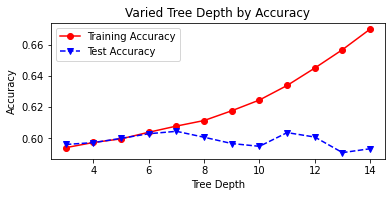
The optimal maximum depth exists where test and training accuracy are both highest (60% and 64%, respectively). This is where depth is equal to 12. Now we can print the classification reports for both the un-tuned and tuned models, noting some improvement in performance.
# Untuned Decision Tree Classifier
untuned_tree = DecisionTreeClassifier(random_state=222)
untuned_tree = untuned_tree.fit(X_train, y_train)

# Predict on test set
untuned_tree1 = untuned_tree.predict(X_test)

# accuracy and classification report
print('Untuned Decision Tree Classifier')
print('Accuracy Score')
print(accuracy_score(y_test, untuned_tree1))
print('Classification Report \n',
       classification_report(y_test, untuned_tree1))

# Tuned Decision Tree Classifier
tuned_tree = DecisionTreeClassifier(max_depth = 12,
                                    random_state=222)
tuned_tree = tuned_tree.fit(X_train, y_train)
# Predict on test set
tuned_tree1 = tuned_tree.predict(X_test)

# accuracy and classification report
print('Tuned Decision Tree Classifier')
print('Accuracy Score')
print(accuracy_score(y_test, tuned_tree1))
print('Classification Report \n',
       classification_report(y_test, tuned_tree1))
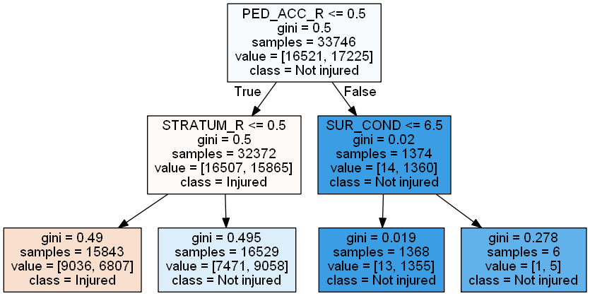
cn = ['Injured', 'Not injured']
reduced_tree = DecisionTreeClassifier(max_depth = 2,
                                      random_state=222)
reduced_tree = reduced_tree.fit(X_train, y_train)
import pydotplus
from IPython.display import Image
# plot pruned tree at a max depth of 2
dot_data = export_graphviz(reduced_tree,
feature_names = X_train.columns,
class_names = cn,
filled = True, out_file=None)
graph = pydotplus.graph_from_dot_data(dot_data)
Image(graph.create_png())
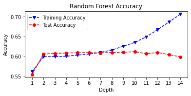
Random Forest Classifier
# Random Forest Tuning
rf_train_accuracy = []
rf_test_accuracy = []
for n in range(1, 15):
    rf = RandomForestClassifier(max_depth = n,
                                random_state=222)
    rf = rf.fit(X_train, y_train)
    rf_pred_train = rf.predict(X_train)
    rf_pred_test = rf.predict(X_test)
    rf_train_accuracy.append(accuracy_score(y_train,
                                            rf_pred_train))
    rf_test_accuracy.append(accuracy_score(y_test,
                                            rf_pred_test))
    print('Max Depth = %2.0f \t Test Accuracy = %2.2f \t \
    Training Accuracy = %2.2f'% (n, accuracy_score(y_test,
                                                  rf_pred_test),
                               accuracy_score(y_train,
                                              rf_pred_train)))
max_depth = list(range(1, 15))
fig, plt.subplots(figsize=(6,2.5))
plt.plot(max_depth, rf_train_accuracy, 'bv--',
         label='Training Accuracy')
plt.plot(max_depth, rf_test_accuracy, 'ro--',
         label='Test Accuracy')
plt.title('Random Forest Accuracy')
plt.xlabel('Depth')
plt.ylabel('Accuracy')
plt.xticks(max_depth)
plt.legend()
plt.show()
# Untuned Random Forest
untuned_rf = RandomForestClassifier(random_state=222)
untuned_rf = untuned_rf.fit(X_train, y_train)

# Predict on test set
untuned_rf1 = untuned_rf.predict(X_test)

# accuracy and classification report
print('Untuned Random Forest Model')
print('Accuracy Score')
print(accuracy_score(y_test, untuned_rf1))
print('Classification Report \n',
       classification_report(y_test, untuned_rf1))

# Tuned Random Forest
tuned_rf = RandomForestClassifier(random_state=222,
                                  max_depth = 12)
tuned_rf = tuned_rf.fit(X_train, y_train)

# Predict on test set
tuned_rf1 = tuned_rf.predict(X_test)

# accuracy and classification report
print('Tuned Random Forest Model')
print('Accuracy Score')
print(accuracy_score(y_test, tuned_rf1))
print('Classification Report \n',
       classification_report(y_test, tuned_rf1))
Model Evaluation
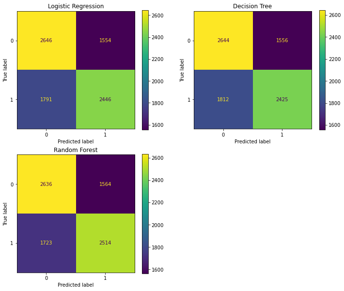
Confusion Matrices
fig = plt.figure(figsize=(12,10))
ax1 = fig.add_subplot(221)
ax2 = fig.add_subplot(222)
ax3 = fig.add_subplot(223)

# logistic regression confusion matrix
plot_confusion_matrix(tuned_lr, X_test, y_test, ax=ax1)
ax1.set_title('Logistic Regression')

# Decision tree confusion matrix
plot_confusion_matrix(tuned_tree, X_test, y_test, ax=ax2)
ax2.set_title('Decision Tree')


# random forest confusion matrix
plot_confusion_matrix(tuned_rf, X_test, y_test, ax=ax3)
ax3.set_title('Random Forest')
plt.show()
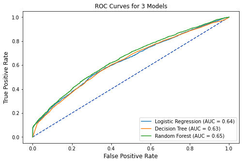
ROC Curves
# extract predicted probabilities from models
tuned_lr_pred = tuned_lr.predict_proba(X_test)[:, 1]
tuned_tree_pred = tuned_tree.predict_proba(X_test)[:, 1]
tuned_rf_pred = tuned_rf.predict_proba(X_test)[:, 1]

# plot all of the roc curves on one graph
tuned_lr_roc = metrics.roc_curve(y_test,tuned_lr_pred)
fpr,tpr,thresholds = metrics.roc_curve(y_test,tuned_lr_pred)
tuned_lr_auc = metrics.auc(fpr, tpr)
tuned_lr_plot = metrics.RocCurveDisplay(fpr=fpr,tpr=tpr,
roc_auc = tuned_lr_auc,
estimator_name = 'Logistic Regression')

tuned_tree_roc = metrics.roc_curve(y_test,tuned_tree_pred)
fpr,tpr,thresholds = metrics.roc_curve(y_test,tuned_tree_pred)
tuned_tree_auc = metrics.auc(fpr, tpr)
tuned_tree_plot = metrics.RocCurveDisplay(fpr=fpr,tpr=tpr,
roc_auc=tuned_tree_auc,
estimator_name = 'Decision Tree')

tuned_rf1_roc = metrics.roc_curve(y_test, tuned_rf_pred)
fpr,tpr,thresholds = metrics.roc_curve(y_test,tuned_rf_pred)
tuned_rf1_auc = metrics.auc(fpr, tpr)
tuned_rf1_plot = metrics.RocCurveDisplay(fpr=fpr,tpr=tpr,
roc_auc=tuned_rf1_auc,
estimator_name = 'Random Forest')

# plot set up
fig, ax = plt.subplots(figsize=(8,5))
plt.title('ROC Curves for 3 Models',fontsize=12)
plt.plot([0, 1], [0, 1], linestyle = '--',
         color = '#174ab0')
plt.xlabel('',fontsize=12)
plt.ylabel('',fontsize=12)

# Model ROC Plots Defined above
tuned_lr_plot.plot(ax)
tuned_tree_plot.plot(ax)
tuned_rf1_plot.plot(ax)
plt.show()
Performance Metrics
# Logistic Regression Performance Metrics
report1 = classification_report(y_test,tuned_lr1,
output_dict=True)
accuracy1 = round(report1['accuracy'],4)
precision1 = round(report1['1']['precision'],4)
recall1 = round(report1['1']['recall'],4)
fl_score1 = round(report1['1']['f1-score'],4)

# Decision Tree Performance Metrics
report2 = classification_report(y_test,tuned_tree1,
output_dict=True)
accuracy2 = round(report2['accuracy'],4)
precision2 = round(report2['1']['precision'],4)
recall2 = round(report2['1']['recall'],4)
fl_score2 = round(report2['1']['f1-score'],4)

# Random Forest Performance Metrics
report3 = classification_report(y_test,tuned_rf1,
output_dict=True)
accuracy3 = round(report3['accuracy'],4)
precision3 = round(report3['1']['precision'],4)
recall3 = round(report3['1']['recall'],4)
fl_score3 = round(report3['1']['f1-score'],4)
table1 = PrettyTable()
table1.field_names = ['Model', 'Test Accuracy',
                      'Precision', 'Recall',
                      'F1-score']
table1.add_row(['Logistic Regression', accuracy1,
                precision1, recall1, fl_score1])
table1.add_row(['Decision Tree', accuracy2,
                precision2, recall2, fl_score2])
table1.add_row(['Random Forest', accuracy3,
                precision3, recall3, fl_score3])
print(table1)
# Mean-Squared Errors
mse1 = round(mean_squared_error(y_test, tuned_lr1),4)
mse2 = round(mean_squared_error(y_test, tuned_tree1),4)
mse3 = round(mean_squared_error(y_test, tuned_rf1),4)

table2 = PrettyTable()
table2.field_names = ['Model', 'AUC', 'MSE']
table2.add_row(['Logistic Regression',
                 round(tuned_lr_auc,4), mse1])
table2.add_row(['Decision Tree',
                 round(tuned_tree_auc,4), mse2])
table2.add_row(['Random Forest',
                 round(tuned_rf1_auc,4), mse3])
print(table2)
Reference
Shmueli, G., Bruce, P. C., Gedeck, P., & Patel, N. R. (2020). Data mining for business
analytics: Concepts, techniques and applications in Python. John Wiley & Sons, Inc.